Spectrum: 3-5x Diffusion Speedup Without Any Training -- The Power of Chebyshev Polynomials
CVPR 2026 paper from Stanford/ByteDance. Chebyshev polynomial feature forecasting achieves 4.79x speedup on FLUX.1, 4.56x on HunyuanVideo. Training-free, instantly applicable to any model.

Spectrum: 3-5x Diffusion Speedup Without Any Training -- The Power of Chebyshev Polynomials
Diffusion models produce stunning images and videos, but they're slow. A 50-step sampling process requires pushing billions of parameters through the network at every single step. Methods like DDIM and DPM-Solver reduce the number of steps, but each step still demands a full network forward pass.
Spectrum, from Stanford and ByteDance (CVPR 2026), takes an entirely different approach. Instead of reducing steps, it skips the network computation at certain steps entirely -- without any additional training. The key insight: model the feature evolution along the diffusion trajectory using Chebyshev polynomials, then forecast features at skipped steps.
The results: 3.47-4.79x speedup on FLUX.1, 3.36-4.56x on HunyuanVideo -- with minimal quality degradation.
Background: Two Directions for Diffusion Acceleration
Making diffusion models faster falls into two categories:
1. Step Reduction
Methods like DDIM, DPM-Solver, and DPM-Solver++ use better ODE/SDE solvers to reduce 50 steps to 20-25. But each step still requires a full network forward pass.
2. Feature Caching/Reuse
Methods like DeepCache (CVPR 2024) reuse features computed at previous steps, allowing some steps to skip the network computation entirely. This reduces the per-step cost rather than the step count.
Spectrum is the latest evolution of the second category. Rather than naively copying previous features, it makes mathematically rigorous predictions.
The Problem with Taylor Expansion
Before Spectrum, TaylorSeer (ICCV 2025) attempted feature prediction using Taylor expansion. The fundamental problem: Taylor expansion is a local approximation. It's accurate near the cached points but errors grow rapidly with distance. When you skip multiple steps, errors compound and image quality degrades significantly.
Think of it this way: Taylor expansion predicts the future by looking at "what just happened recently." It's like predicting stock prices will keep rising because they rose yesterday -- reasonable short-term, but unreliable for longer horizons.
Spectrum's Core Idea: Global Spectral Approximation
Spectrum's key insight is elegant:
View each feature channel's evolution along the diffusion sampling trajectory as a function over time, and approximate it with a linear combination of Chebyshev polynomials.
Chebyshev polynomials are orthonormal bases known to provide optimal function approximation. The critical advantages:
- Global approximation: Captures the pattern across the entire time interval
- Non-compounding errors: Approximation error is independent of step size (Theorem 3.3)
- Stable fitting: Ridge regression prevents overfitting
If Taylor is a "local weather forecast," Spectrum is "climate pattern modeling." By capturing the overall trend, it can accurately predict further into the future.
Algorithm Details
Step 1: Timestep Mapping
Map diffusion timesteps to the Chebyshev domain [-1, 1]:
tau = g(t) = 2t - 1
Step 2: Chebyshev Polynomial Approximation
Approximate each feature channel h_i(t) as a linear combination of M Chebyshev polynomials:
h_i(t) ≈ c_0 * T_0(tau) + c_1 * T_1(tau) + ... + c_M * T_M(tau)
The Chebyshev polynomials of the first kind:
- T_0(x) = 1
- T_1(x) = x
- T_2(x) = 2x² - 1
- T_3(x) = 4x³ - 3x
- T_4(x) = 8x⁴ - 8x² + 1
The default setting uses M=4 (4th degree polynomial).
Step 3: Ridge Regression Coefficient Fitting
Using feature values from steps where actual forward passes were computed, fit the coefficient vector C:
C = (Φ^T·Φ + λ·I)^{-1} · Φ^T · H
Where:
- Φ is the Chebyshev basis evaluation matrix at computed steps
- H contains the actual feature values at those steps
- λ=0.1 is the regularization strength (prevents overfitting)
Step 4: Feature Forecasting
At steps in the forecast set V (skipped steps), predict features using the fitted coefficients:
h(t_j) = φ(g(t_j)) · C
A simple matrix-vector product replaces the entire network forward pass.
Step 5: Adaptive Scheduling
Steps are divided into two sets:
- U (actual set): Steps with full network forward passes where coefficients are updated
- V (forecast set): Steps where features are predicted via Chebyshev approximation
The flex_window parameter (α) controls adaptive window scaling. As more data points are collected, the forecast horizon grows, allowing more computation to be skipped in later steps.
Error Bounds: Why This Beats Taylor
The theoretical core is Theorem 3.3:
ε_M = ||f - p_M||_∞ ≤ (2B / (ρ - 1)) · ρ^{-M}
This bound is independent of step size. Increasing M (polynomial degree) reduces error exponentially. In contrast, Taylor expansion errors compound with the skip horizon.
Empirically confirmed: Feature RMSE at step 50 is Spectrum 0.1674 vs Taylor 0.2510 (33% lower).
Results
Text-to-Image
FLUX.1-dev (50-step reference):
| Method | NFE | Speedup | PSNR↑ | SSIM↑ | LPIPS↓ |
|---|---|---|---|---|---|
| Spectrum (α=0.75) | 14 | 3.47x | 24.32 | 0.854 | 0.217 |
| Spectrum (α=3.0) | 10 | 4.79x | 22.21 | 0.788 | 0.261 |
| TaylorSeer (N=4) | ~16 | 3.13x | 22.31 | 0.841 | 0.215 |
| TaylorSeer (N=6) | ~12 | 3.99x | 17.41 | 0.708 | 0.389 |
Stable Diffusion 3.5-Large:
| Method | NFE | Speedup | PSNR↑ | SSIM↑ | LPIPS↓ |
|---|---|---|---|---|---|
| Spectrum (α=0.75) | 14 | 3.21x | 17.83 | 0.743 | 0.305 |
| Spectrum (α=3.0) | 10 | 4.32x | 15.68 | 0.620 | 0.430 |
Text-to-Video
HunyuanVideo:
| Method | NFE | Speedup | PSNR↑ | SSIM↑ | LPIPS↓ |
|---|---|---|---|---|---|
| Spectrum (α=0.75) | 14 | 3.36x | 27.77 | 0.842 | 0.209 |
| Spectrum (α=3.0) | 10 | 4.56x | 25.39 | 0.779 | 0.273 |
Wan2.1-14B:
| Method | NFE | Speedup | PSNR↑ | SSIM↑ | LPIPS↓ |
|---|---|---|---|---|---|
| Spectrum (α=0.75) | 14 | 3.40x | 22.78 | 0.749 | 0.222 |
| Spectrum (α=3.0) | 10 | 4.67x | 21.24 | 0.694 | 0.265 |
| TaylorSeer (N=6) | ~12 | 3.94x | 17.24 | 0.585 | 0.367 |
The gap is especially pronounced in video generation, where each step's cost is higher due to the larger number of frames, making feature prediction accuracy critical.
Supported Models
Spectrum works across both U-Net and Transformer/DiT architectures:
| Model | Architecture | Task |
|---|---|---|
| FLUX.1-dev | DiT (Transformer) | Text-to-Image |
| SD 3.5-Large | MMDiT | Text-to-Image |
| SDXL | U-Net | Text-to-Image |
| HunyuanVideo | DiT | Text-to-Video |
| Wan2.1-14B | DiT | Text-to-Video |
Architecture-agnostic operation is a major advantage. By applying feature caching only to the last block, Spectrum minimizes dependency on model internals.
Hyperparameter Guide
| Parameter | Default | Role |
|---|---|---|
| w | 0.5-1.0 | Blending factor (1.0 = pure Chebyshev) |
| λ (lam) | 0.1 | Ridge regression regularization |
| M (m) | 4 | Number of Chebyshev basis functions |
| N (window_size) | 2 | Initial fitting window size |
| α (flex_window) | 0.75 | Adaptive window scaling |
Practical tips:
- α=0.75 prioritizes quality, α=3.0 prioritizes speed
- λ too small (0.001) causes overfitting, too large (10) causes underfitting
- M=4 is the sweet spot between accuracy and computational cost
Comparison with Other Methods
| Category | Representative | Principle | Relation to Spectrum |
|---|---|---|---|
| Step reduction | DDIM, DPM-Solver | Better ODE solvers | Complementary -- can combine |
| Naive caching | DeepCache | Copy previous features | Spectrum strictly superior |
| Local prediction | TaylorSeer | Taylor expansion | Spectrum wins via non-compounding error |
| Spectral prediction | Spectrum | Chebyshev polynomial fitting | -- |
Key point: Spectrum is orthogonal to step-reduction methods. You can apply both simultaneously -- reduce step count AND reduce per-step cost for compounding acceleration.
Hands-On: Accelerating SDXL with Spectrum
A practice notebook using the official code (github.com/hanjq17/Spectrum) is available separately, covering:
- Loading SDXL and baseline generation
- Applying Spectrum and comparing speed/quality
- Visualizing results across hyperparameter settings
- Analyzing Chebyshev approximation error
Conclusion
Spectrum introduces a new paradigm for diffusion model acceleration:
- Training-free: Instantly applicable to any pretrained model
- Theoretically grounded: Non-compounding error bound from Chebyshev approximation
- Universal: Supports both U-Net and DiT architectures, both image and video
- Practical: Up to 4.79x speedup, bringing real-time generation closer to reality
Combined with step-reduction methods, even greater acceleration is achievable. A ComfyUI plugin is already available for immediate integration into production workflows.
References:
Subscribe to Newsletter
Related Posts
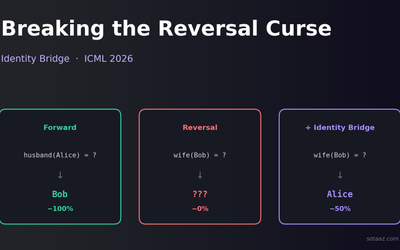
Breaking the Reversal Curse with Identity Bridges — the ICML 2026 fix that shouldn't work but does
LLMs trained on "Alice's husband is Bob" famously fail on "Bob's wife is?" — the reversal curse. A new ICML 2026 paper fixes it by adding one weird kind of self-referential example to the training set. The naive version doesn't work; the right version does.

MIRAGE — Do Multimodal AIs Actually "See" Images?
GPT-5.1, Gemini 3 Pro, and Claude Opus 4.5 retain 70-80% of benchmark scores without any image input. A 3B text-only model outperforms all multimodal models and radiologists on chest X-ray benchmarks. Stanford MIRAGE paper review.

InternVL-U: Understanding + Generation + Editing in One 4B Model -- A New Standard for Unified Multimodal AI
Shanghai AI Lab's InternVL-U. A single 4B parameter model handles image understanding, generation, editing, and reasoning-based generation. Decoupled visual representations outperform 14B BAGEL on GenEval and DPG-Bench.