Can a Text Model Match Photos Without Seeing Them? Rerunning Yann LeCun’s JEPA Paper
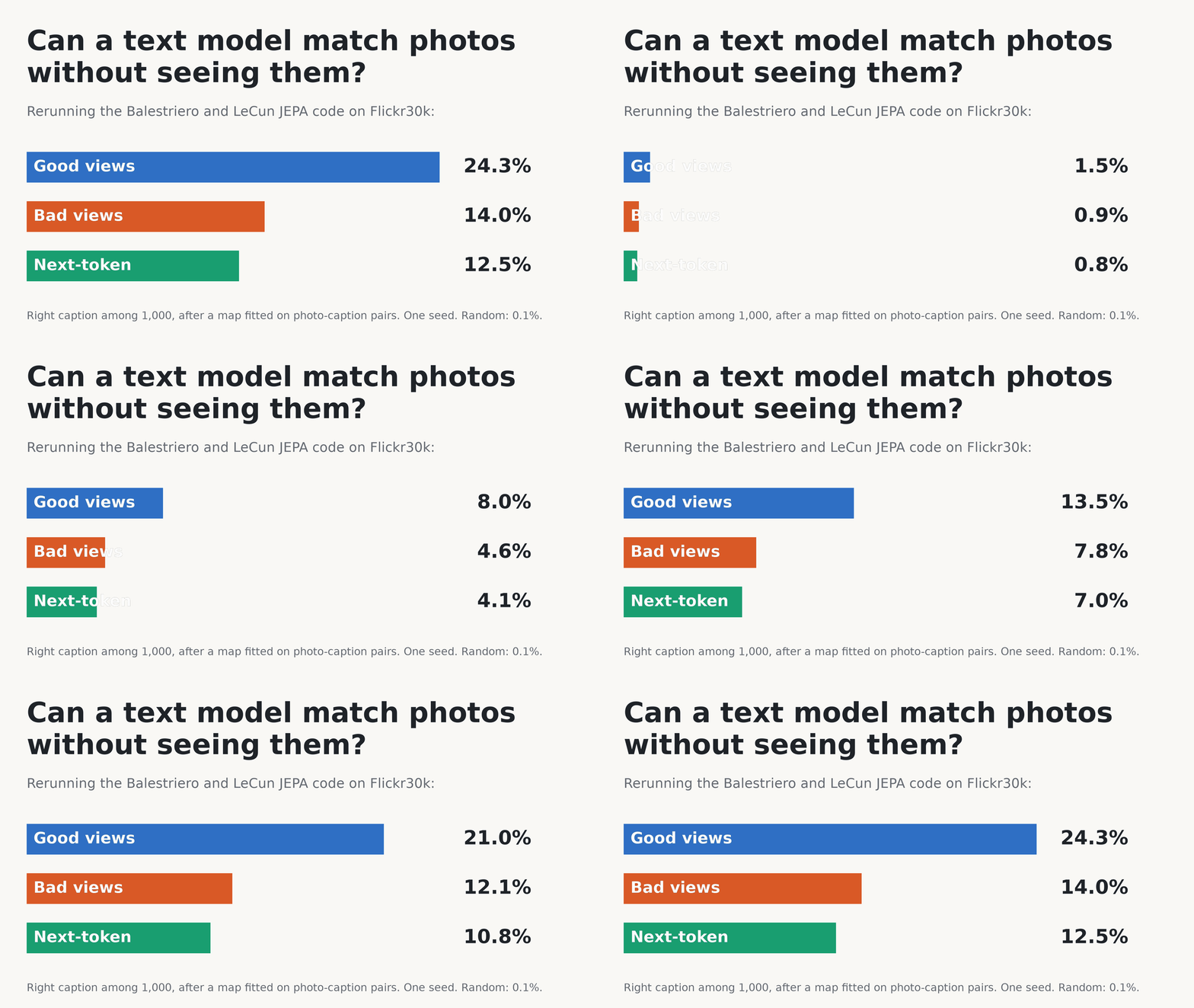
We reran Balestriero and LeCun’s JEPA code on Flickr30k. A text encoder trained on different captions of one photo retrieved the correct caption 24.3% of the time, versus 12.5% for next-token prediction, after fitting a map to DINOv2. We explain the setup and its limits.
Can a Text Model Match Photos Without Seeing Them? Rerunning Yann LeCun’s JEPA Paper
Can a text model that never receives photos as training inputs help choose the right caption for a photo? In Proving and Improving the Platonic Representation Hypothesis with JEPAs, Randall Balestriero and Yann LeCun study how separately trained text and image models come to organize information in similar ways. We ran the authors' code on a small experiment.
The task is to match each test photo to its caption among 1,000 candidates. An image encoder turns the photo into a vector, a list of numbers representing its features. A text encoder does the same for each caption. After fitting one linear map between their vector spaces, we choose the caption whose vector is closest to the photo's. The text encoder learns from captions without receiving the photos themselves.
We changed how that text encoder learns. Different captions of one photo can describe the same scene in different words: "a dog is running" and "a puppy is chasing a ball," for example. Training their vectors to be close may encourage the model to keep the scene they share. The paper compares this with matching pieces of a single caption, and with next-token prediction, the objective used to train LLMs.
Here is how often our models chose the correct caption as their top match. Random selection gets 0.1%.
| Text encoder training | Correct top match |
|---|---|
| Match views drawn from the different captions of one photo | 24.3% |
| Match views cut from one caption | 14.0% |
| Predict the next token | 12.5% |
The paper calls the first two settings "good views" and "bad views." A view is an input made for training. The distinction is where it comes from: good views draw from the captions grouped under one photo; bad views draw from a single caption. We use the paper's names below to make the connection to its code clear.
The map between the two encoders matters. We fitted it on 1,014 photo-caption pairs after training, then scored it on 1,000 other pairs. The 24.3% result includes this calibration. Although the text encoder receives no photos, making good views also requires knowing which captions belong to the same photo. There is pairing information in the experiment.
We kept the pretrained image encoder DINOv2 fixed and trained a 33M-parameter text encoder three ways on the same pool of 145,000 Flickr captions: 29,000 photos, five captions each. All three ran for 200 epochs. A good-view sample draws its views from all five captions; the other two settings read one caption per photo in each epoch. Equal epochs therefore do not mean equal token counts. Next-token prediction sees fewer tokens per step, which the paper also notes.
The order of the scores matches the paper, but this is one seed on a small dataset. The last two differ by 1.5 percentage points, with a 95% interval of −0.9 to 4.0 points, so this run cannot separate them.
The paper calls next-token prediction "a remarkably inefficient route to platonic representations," referring to the data and model scale needed for separately trained models to develop similar representations. This is not a claim about overall LLM ability. Our scores at equal epochs do not test that efficiency claim. We did not rerun the web-scale experiments behind "42 times fewer samples" or the comparisons with large LLMs; those results are identified as the paper's below.
Here are examples of the captions the models choose. These six images are new: we generated them with FLUX.1-schnell, so no encoder trained on them. Each caption is the top match out of 29,909 MS COCO captions.
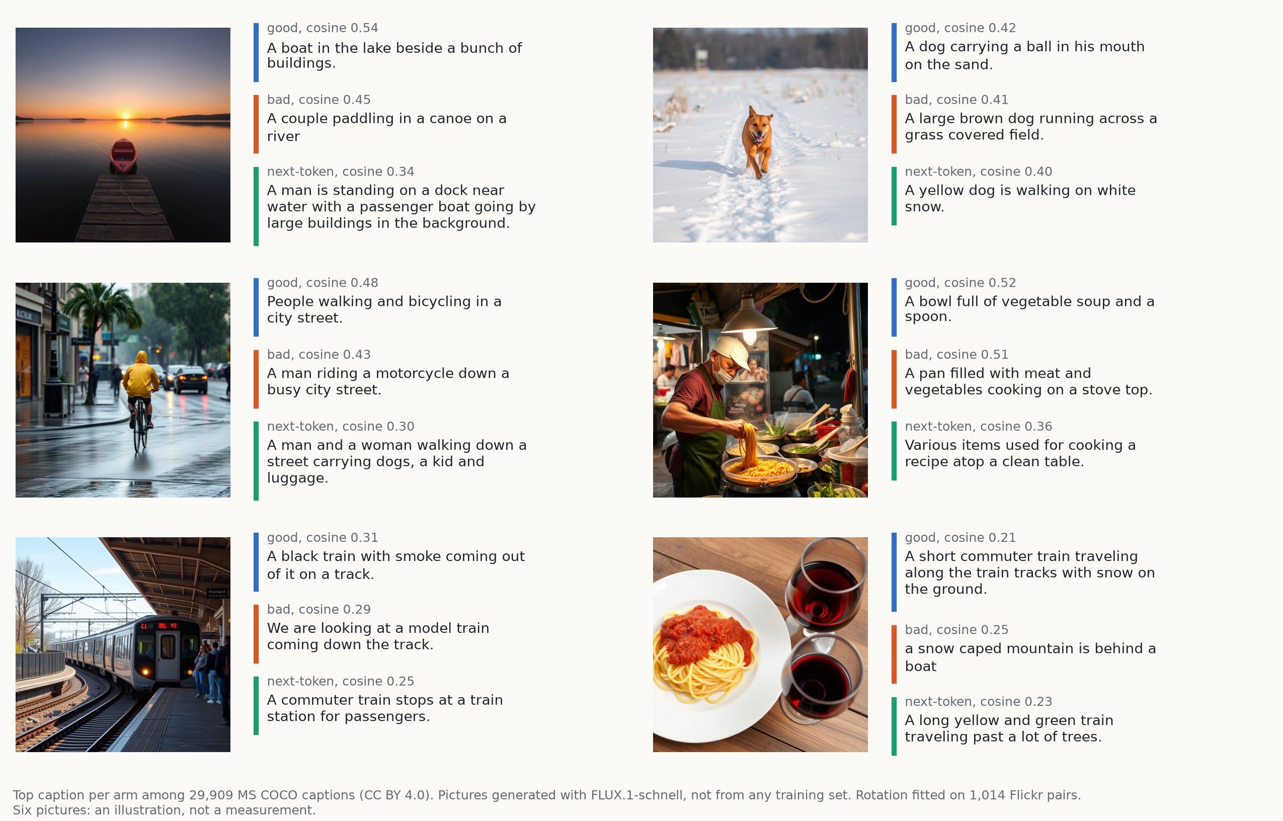
Treat this as an illustration, since six pictures cannot rank anything. The boat, the street and the train land close. On the dog, next-token prediction is the one that reads the snow. Spaghetti defeats all three, returning trains and a mountain. The candidate pool is not to blame: 50 of its captions mention pasta, spaghetti or noodles. Only 54 of the 145,000 Flickr training captions do, which points to scarce pasta and noodle text, but that does not explain it by itself. On the noodle stall, the good-view encoder's top two captions are about soup and a chef, at cosines of .52 and .51 (the figure shows only the first). We did not test why the plate fails. Its cosines are .21 to .25, against .25 to .31 for the train and .34 to .54 for the boat, so the score alone does not mark a failure.
What the paper proves
The Platonic Representation Hypothesis, from Huh et al., proposes that models trained on different data converge toward similar representations. Here, a representation is the vector a model uses to describe an input. Agreement need not mean identical vector coordinates: it can mean similar relationships between inputs, including which ones are close together.
The new paper proves a conditional version of this idea for a particular setting of joint-embedding predictive architectures (JEPAs). In the setting studied here, training brings the vectors of different views of the same thing close together. A separate constraint prevents collapse, the useless solution where every input maps to one point.
The setup has a hidden world. Each state of the world can appear as a photo or as a caption, and each appearance carries its own extra detail, which the paper calls nuisance: the camera angle, or the choice of words.
Theorem 1. If two modalities train JEPAs on the same distribution of positive pairs (inputs trained to be close) over world states, and the solution of that problem is unique up to rotation, then the two encoders agree up to one rotation. That means one common change of coordinates for all their vectors. The proof is short. If a rendering is injective (no two states look the same), it only changes coordinates, so training an encoder on observations is the same problem as training one directly on world states. Two modalities are then solving one problem, which has one answer, up to rotation.
The hypotheses matter: a finite world, injective renderings, population optima. The authors say no experiment meets them exactly. Proposition 1 gives a concrete case where uniqueness holds: squared loss with whitening, which sets the embedding mean to zero and covariance to the identity. When the spectrum has a gap (μₖ > μₖ₊₁), its solution is the top eigenvectors of the positive-pair kernel (Laplacian eigenmaps). Uniqueness for SIGReg, the regularizer used in the experiments, is assumed and not proved.
Why the first two moments cannot find the rotation. Proposition 2 says the first two moments of unpaired data cannot identify the rotation, because whitened embeddings look the same under every rotation. With equal widths, k pairs in general position determine it.
Why views matter. Theorem 3 sets a floor on the mismatch: the less of an embedding that the world state explains, the larger the best-rotation error must be. Proposition 3 then separates two ways of making views.
- Good views are different observations of one state. Two captions of the same photo share the scene and can differ in wording. In the idealized setup, observation-specific wording averages out, leaving the shared scene information.
- Bad views are corruptions of a single observation. Two crops of one caption share its wording, so wording is a valid thing to keep. If the nuisance is strong enough, it takes up embedding directions that the scene needed.
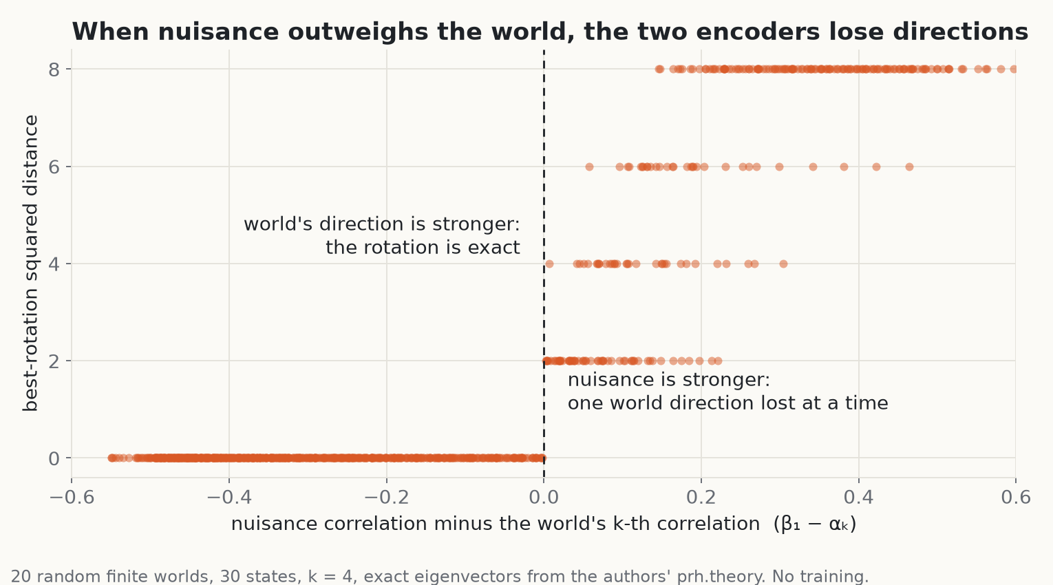
Written with correlations, a bad view spends r ≥ 1 directions on nuisance exactly when the strongest nuisance correlation β₁ exceeds the k-th world correlation αₖ.
Proposition 4 adds next-token prediction. Its softmax loss can be written as a prediction term plus a log-partition term that resists collapse, and its positives are a prefix and its continuation, which come from one text. That makes it bad-view shaped. The authors flag the application as heuristic, "a prediction to test".
We checked the threshold with the authors' prh/theory.py, using exact eigenvectors and no training: 20 random worlds with 30 states and k = 4, for 800 grid points. With good views, the largest absolute error was 5.3e-15. Under the bad-view threshold, all 545 points have an absolute error of at most 7.1e-15. Above it, all 255 points lost at least one direction, and the error equals 2r to within 6e-14. In this setup each lost direction costs exactly 2. We left out the 20 rows where a corruption keeps the nuisance entirely. There all four directions go to the nuisance and the encoder keeps no world state, so the error is 2k = 8, which is 2r with r = 4. The authors' nuisance_directions returns r = 3 on these rows: the eigenvalues tie exactly, and its sort drops a nuisance direction instead of the trivial constant one. Dropping the constant direction explicitly gives r = 4 on all 20.
The paper, mapped to the code
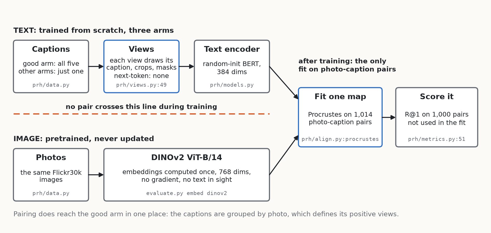
In our rerun, no training loss directly matches a text vector to an image vector. The map between them is fitted on photo-caption pairs after training. Good-view training still uses the grouping of captions by photo to choose its inputs.
| Paper | Code | What it does |
|---|---|---|
| Good views vs bad views (Prop. 3) | prh/views.py, TextView.__call__, prh/data.py, pick | A list of captions or a single one |
| JEPA objective with identity predictor | stable_pretraining/methods/lejepa.py, _compute_loss | Pull every view to the mean of the global views |
| Anti-collapse | SlicedEppsPulley, same file | Push projections toward an isotropic Gaussian |
| Next-token as a JEPA (Prop. 4) | prh/forward.py, next_token | Tied softmax over the vocabulary |
| The one rotation (Thm. 1, Prop. 2) | prh/align.py, procrustes | SVD of the pair cross-covariance |
| The evaluation | prh/metrics.py, alignment, recall | Fit on some pairs, score on others |
| The theory, executable | prh/theory.py, tests/test_theory.py | Finite worlds as NumPy arrays |
The docstrings use a different numbering in places. prh/forward.py calls next-token "Prop. 2", which is Proposition 4 in arXiv v1. We use the arXiv numbers here.
The line that separates good from bad
if isinstance(ids, list):  # good views: each view draws its own caption of the image
    ids = ids[torch.randint(len(ids), ()).item()]
This is prh/views.py, lines 49-50. The flag --caption-views makes pick in prh/data.py return all five captions of a photo. Each of the eight views then draws a caption at random, so two views can land on the same one. Without the flag, pick returns one caption and all eight views cut from it. Everything after that line is shared: a random span, 15% of tokens masked, two global views keeping 50-100% of the caption and six local views keeping 15-50%.
The why follows from Proposition 3. The good and bad arms get the same crops and the same masking, so the only thing that changes is what the views have in common. That is what the proposition says matters, so the code changes only that.
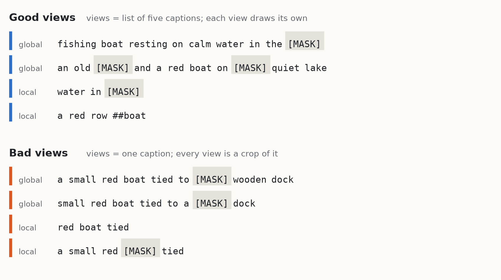
These views come from the real transform, run on five captions we wrote for the example. Look at the two groups. All four bad views come from one sentence, so they can agree by keeping its exact words, such as "red" and "tied". Good views can come from different sentences, so retaining one sentence's exact words is less useful for matching them.
This is also where "without seeing them" needs its caveat. No photo reaches the text encoder, but the good arm has to know which captions describe one photo. The paper explicitly identifies three places where pairing information enters: the definition of positives, the fitted linear map, and, on the web-image texts, captions generated by an image captioner. Training without a cross-modal loss still uses these correspondences.
The loss brings view vectors together
centers = all_projected[:n_global].mean(0)
inv_loss = (centers.unsqueeze(0) - all_projected).square().mean()
sigreg_loss = sigreg(all_projected.reshape(-1, all_projected.size(-1)))
loss = inv_loss + lamb * sigreg_loss
This comes from the stable-pretraining library, lejepa.py, lines 268-273. The target is the mean vector of the two longer inputs, called global views, and every view vector is pulled toward it. There is no learned predictor, which matches the paper's analysis: the predictor is the identity. Learned or action-conditioned predictors, the kind often associated with JEPAs, are not covered by these theorems.
Left alone, the invariance term has a perfect solution, which is to map everything to one point. SIGReg blocks it by testing whether embeddings look like an isotropic Gaussian. A test in hundreds of dimensions would be hard, so it projects onto 1,024 random unit directions, redrawn every step, and compares each one-dimensional result with a standard normal through the characteristic function at 17 points. This plays the role that whitening plays in Proposition 1, and the Gaussian target is stricter than whitening, since whitening only fixes the first two moments.
One detail is easy to miss. The statistic is multiplied by the number of samples ((err @ self.weights) * N * self.world_size), so lamb alone does not set its strength. The repo's docs/reproduce.md says this directly: at the pinned revision, the effective weight is proportional to the per-GPU batch, and the 940M-image run at 128 per GPU with weight .02 matches --lamb 0.01 at 256 per GPU. self.world_size is the process count if distributed training is already running when the loss is built, and 1 otherwise; we did not check which applied in the authors' runs. N counts every view in the batch, so the number of views moves the effective weight too.
The paper shows where this matters. R@1 is the caption score from the opening; mutual 10-NN, a neighbour-overlap score, and the WIT benchmark are explained below. A seed at twice the effective weight reached .121 on WIT mutual 10-NN, where the other three average .184, while its Flickr R@1 with a 30k-pair map hardly moved (.477 against .478). On Flickr30k with the 1,014-pair map, batch 512 gives R@1 .241 against .246 at the default. The authors draw the conclusion themselves: "at this scale WIT is sensitive to the SIGReg weight, which our ablations on Flickr captions did not reveal". Larger changes do show on Flickr: with gradient clipping and one seed each, λ = .05 collapses and λ = .1 reaches .202. If you change the batch size, the same .02 is a different experiment, even when your metric does not show it.
Next-token prediction in two lines
logits = h[:, :-1] @ self.backbone.bert.embeddings.word_embeddings.weight.T
loss = F.cross_entropy(logits.flatten(0, 1).float(), tokens[:, 1:].flatten(), ignore_index=self.backbone.pad_id)
The logits use the input word embeddings as the output head, so the dot product between a hidden state and a word's embedding is the score. Expanding cross-entropy gives −⟨h, e_y⟩ + log Σ e^⟨h, e_v⟩: a pull toward the next token, plus a term that stops h from collapsing. That is the JEPA shape of Proposition 4, and writing the loss this way makes the mapping visible. This arm has no views at all, and reads a whole caption.
The map between the encoders
u, _, vt = torch.linalg.svd(a.T @ b, full_matrices=False)
return u @ vt
This is orthogonal Procrustes in prh/align.py, and it is the only thing fitted on pairs. The catch is the widths. DINOv2 ViT-B outputs 768 dimensions and the default text encoder 384, so the map is 768 by 384 with orthonormal columns. It reduces the image vectors to 384 dimensions, rather than rotating within a space of equal width. The repo's docstring says "we keep calling it the rotation". The paper says so in its own text, calling this "a case the theory does not cover" and giving 0.22M free parameters. The exact count is 768·384 − 384·385/2 = 220,992, fitted on 1,014 pairs, and that gap appears to show in our numbers below.
The scoring is careful in two places
rank = (s >= s.diag()[:, None]).sum(1) - 1The >= in recall counts ties against the true pair. If an encoder collapsed to one point, every score would tie exactly and the true caption would rank last, for a score of 0. With >, the same encoder would score perfectly. The docstring describes this case as scoring at chance, but on exact ties this line gives 0. In alignment, both the means and the map are computed only on non-test rows, so test pairs cannot leak into the fit.
Our rerun
R@1 here means: for each of 1,000 test photos, is its own caption the top match among those 1,000 captions? Chance is .001. We ran the repo's default arguments with seed 0 on one A100. The three arms shared the GPU and all finished in under 3 hours 50 minutes. We used the pinned stable-pretraining revision and newer versions of the other libraries than the authors did (torch 2.15, against PyTorch 2.11 in the repo's reproduction guide).
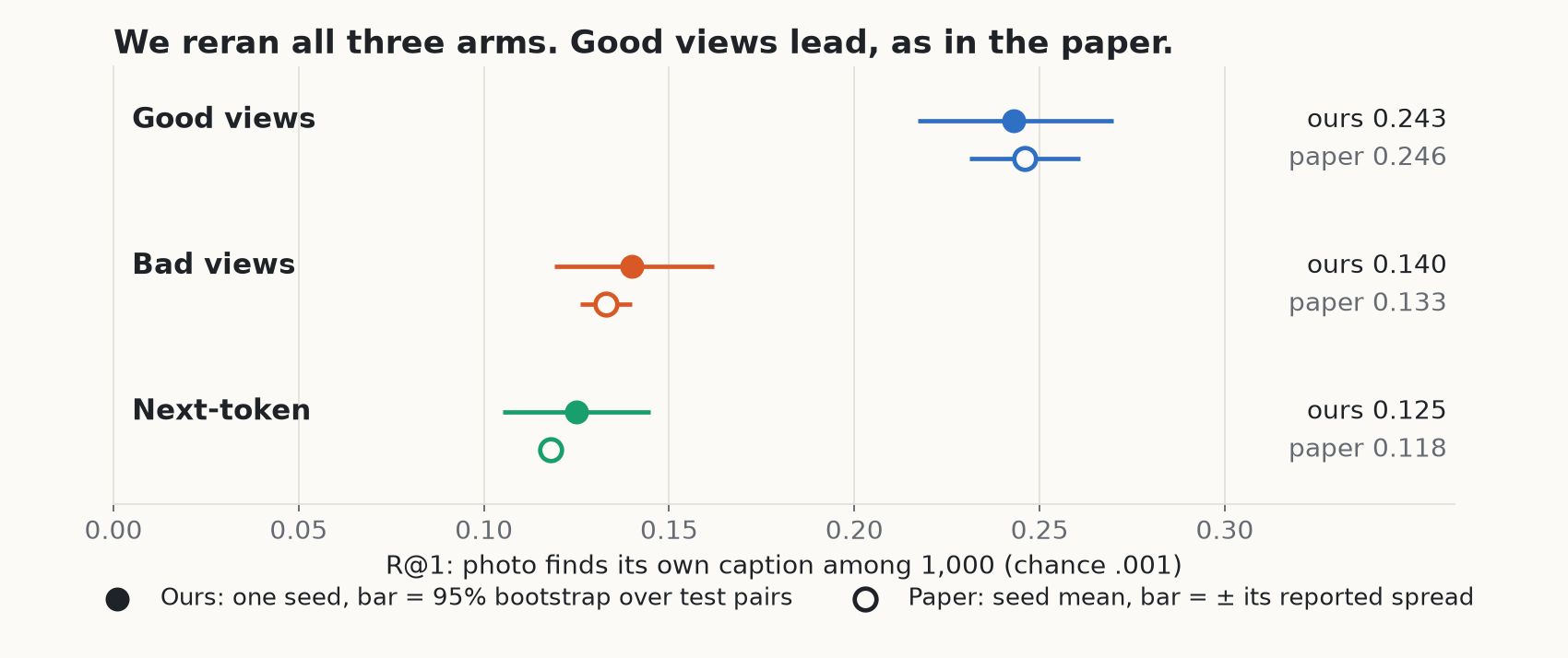
| Arm | Ours R@1 [95% over test pairs] | Paper R@1 | Ours mutual 10-NN | Paper mutual 10-NN |
|---|---|---|---|---|
| Good views | .243 [.217, .270] | .246 ± .015 | .233 | .232 ± .006 |
| Bad views | .140 [.119, .162] | .133 ± .007 | .136 | .132 ± .001 |
| Next-token | .125 [.105, .145] | .118 ± .002 | .121 | .122 ± .001 |
The gap between good views and bad views is what held clearly: +.103, with a paired bootstrap interval of [.075, .131]. Against next-token it is +.118 [.089, .147]. Mutual 10-NN is the average share of each item's 10 nearest cosine neighbours that the two encoders have in common, so it fits no map at all. Its chance level is near .01, and it gives the same order.
Three things in this table need care. It is one seed, so our intervals only cover which test pairs were drawn, and say nothing about training variation. One seed cannot separate bad views from next-token: that difference is +.015 [−.009, .040]. And at three decimals, two of our numbers fall outside the paper's mean ± half-range over three seeds: next-token R@1, .125 against .118 ± .002, and bad-view mutual 10-NN, .136 against .132 ± .001. For R@1, the paper's mean is still inside our test-pair interval.
We also ran two controls. A random orthonormal map scores about .001 on all three arms, and so does a map fitted on shuffled pairs. So the score does come from the pairing.
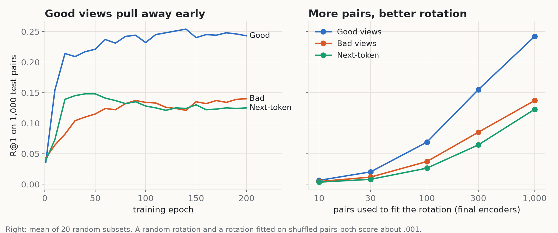
The left panel adds a better floor than chance. After one epoch all three arms already score about .04 (.036, .043, .039). So a barely trained encoder gets far past .001 with a fitted map, and that is the honest place to start reading the curves. The good-view curve reaches its highest value, .254, at epoch 140 (we count epochs from 1) and then wobbles; we report the last epoch, .243, as the paper does.
Next-token behaves differently. It peaks at .148 around epochs 40 to 50, then falls to .125 by the end, so the last epoch is not its best. The paper noticed this too: stopping at its lowest validation loss, epoch 29 in the paper's numbering, gives .134, and even choosing its best checkpoint on the test pairs gives at most .146. Our peak of .148 is close to that, and still far below the good-view arm.
The right panel shows the fit getting better as we add pairs, up to the 1,000 we have. On the 1,014 pairs it was fitted on, the same map scores .927, .879 and .968, for good, bad and next-token. That gap between fit-pair and test scores is consistent with overfitting: the map has 220,992 free parameters and is estimated from 1,014 pairs. It also means .243 is limited partly by the fit. The paper reports that fitting on all 30,000 Flickr train and validation pairs raises the good-view encoder to .346, against .207 and .213 for the other two arms and .48 to .49 for two reference encoders trained on far more data. We did not rerun that fit.
What the paper claims at scale
We did not rerun this part, and the numbers below are the paper's. The benchmark changes to WIT-1024, from Huh et al., scored by mutual 10-NN with frozen DINOv2. That is the alignment measure, with no fitted map, and each score takes the best pair of layers.
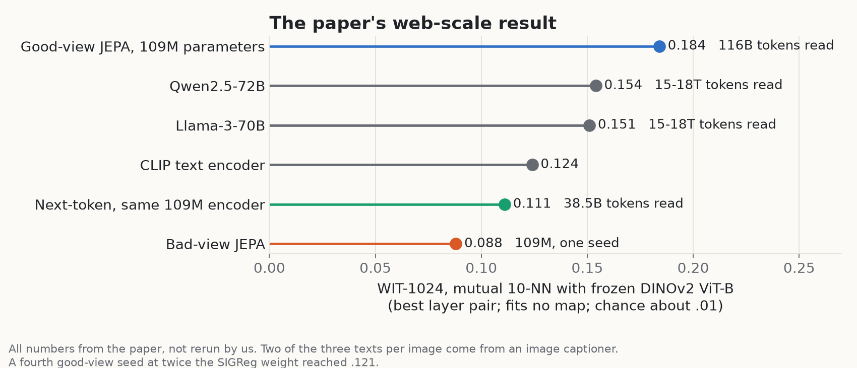
A 109M-parameter good-view encoder reads the texts of 940M web images and scores .184. That is above Qwen2.5-72B (.154) and Llama-3-70B (.151), which were trained on 15 to 18 trillion tokens, against 116 billion here. The authors state these caveats, and they belong with that number.
- Two of the three texts per image are written by an image captioner, LLaVA on LLaMA-3-8B, which sees images through CLIP ViT-L/14. Without any image captioner, good views on the texts of 2.24M images reach .060, against .107 with captioner text on the same images. The comparisons with language models and CLIP's text encoder therefore include the contribution of image-captioner text. Comparing good and bad views on identical texts holds that source of information fixed.
- The fourth seed mentioned above reached .121. All four seeds average .168, still above every language model they scored. The authors say they chose the first run's weight for every other 940M run after seeing this result, "so that weight was selected on WIT".
- Hyperparameters were tuned only for good-view JEPAs, and at least 43 of the 1,024 WIT captions appear in the training texts (removing them changes the score by at most .002).
The headline "42 times fewer samples" compares .109 for good views at 21.6M samples against .111 for next-token at 900M, on the same 109M encoder. The tokens differ by 14 times, 2.77B against 38.52B, because a good-view sample reads three texts. The authors disclose the limits in the same sentence: "we scored no earlier next-token checkpoint", and each run uses the recipe of its scale (learning rate 1e-4 and batch 256, against 2e-4 and 2,048). So the next-token run may have reached .109 before 900M samples, and 42 is measured against the one next-token checkpoint they scored. The same passage reports a higher Flickr R@1, .388 against .335, and at matched samples a larger gap: .108 against .071 at 21.6M samples for the 33M encoder.
One more table comes from the paper (Table 7), whose numbers ship in the repo as paper/data/text_sources.csv. These are means of three seeds at 50M images.
| Texts | Views | WIT mutual 10-NN | R@1 (30k-pair map) |
|---|---|---|---|
| All three | Good | .125 | .376 |
| All three | Bad | .063 | .290 |
| LLaVA only | Good | .096 | .386 |
| LLaVA only | Bad | .092 | .325 |
| Alt-text only | Bad | .056 | .199 |
The table's caption in the paper says that with the same texts, good views double alignment. That fits the all-three row. On LLaVA-only text the WIT gap almost closes, with seeds touching at .093, while the R@1 gap stays. On alt-text at 2.24M images, the paper reports that good views from a text-only paraphrase still beat bad views, .060 against .055 on WIT and .233 against .180 on R@1. The authors do note that "the data matter even with bad views, and the views matter with any texts", and this table shows how much the answer depends on which metric and texts you pick.
Does the effect also appear on video data?
The paper compares good and bad views on video clips from MSR-VTT, training an image model and a text model from scratch. We did not rerun this experiment, and it has no next-token arm.
Good views use different frames of a clip and different descriptions of it. Bad views use crops of one frame and spans of one description. On mutual 10-NN, the scores are .067 and .039 over three seeds. Chance is .01. These are neighbourhood-overlap scores, not caption-retrieval percentages like the 24.3% above.
Most of the gain comes from the text side: .059 with good text views alone, .043 with good image views alone. The paper calls the image-side effect small. On another metric, R@5, changing the image side to good views lowers the score: .099 versus .105 with good text views, and .063 versus .072 with bad text views.
Where this stops
The authors list these limits themselves. The theorems are about idealized worlds. Experiments use LeJEPA, not the squared-loss solution of Proposition 1, and DINOv2 is itself a bad-view encoder under the paper's own definition, along with the authors' image encoders outside MSR-VTT. A good view also needs someone to know which texts describe one scene. That is available in captioned datasets. In our reading, it is not free in general.
From our side: one seed, one dataset, three text arms compared with frozen DINOv2 only, and a demo with six pictures. We did not run the paper's image JEPA or caption-pair arms, and we did not test the captioner, the pair-free ImageNet-100 results or the scaling law.
What we take from the rerun is narrow and held up: on Flickr30k, with this code, changing what the views share moved R@1 from .140 to .243, close to the paper's .133 and .246.
To run it yourself, install the repo with stable-pretraining at revision ab836bf, download Flickr30k (about 8 GB), and then:
python train.py --modality text --caption-views        # good views
python train.py --modality text                        # bad views
python train.py --modality text --objective ntp        # next-token
python evaluate.py embed dinov2 runs/ref/flickr_dinov2
python evaluate.py align runs/ref/flickr_dinov2 <text run> --last
The repo's tests run on a CPU and need no dataset, though some download tokenizers. For us, pytest -m "not slow" gave 129 passed, 6 failed and 2 skipped. Five failures are plot tests stopped by a missing cm-super LaTeX package on our machine. The sixth, the unbiased CKA test, stops inside pytest.approx with TypeError: iteration over a 0-d tensor; we did not fix it, and our scores use mutual 10-NN and R@1, not CKA. tests/test_theory.py alone passes all 37, including test_thm1_two_modalities_with_the_same_positives_agree_up_to_rotation. Start there if you want to see Theorem 1 hold before spending GPU hours.
Images generated with FLUX.1-schnell. Captions in the demo are from MS COCO (CC BY 4.0). We do not republish Flickr30k photos. Code quoted from the MIT-licensed prh-proof repository at commit a2b9949, and stable-pretraining.