TurboQuant Explained — Google's Extreme KV Cache Compression Algorithm
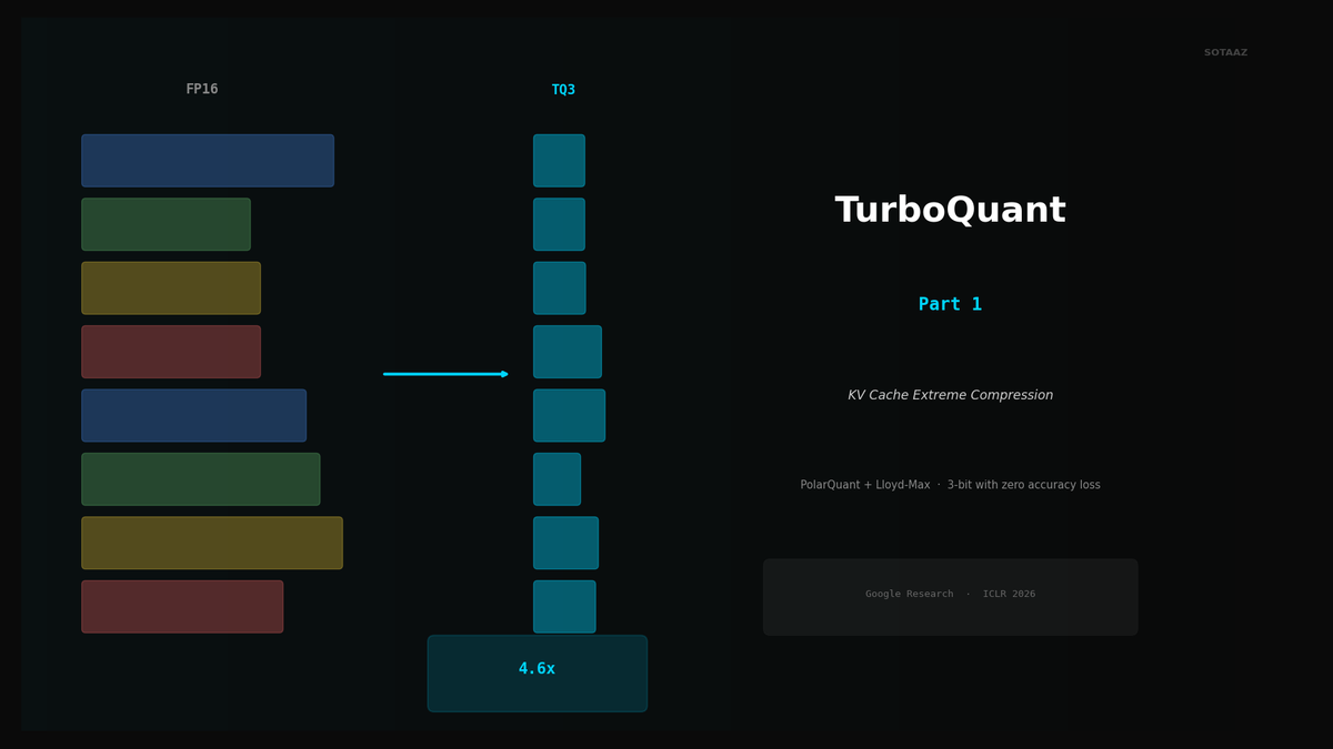
Compress KV cache to 3-bit with PolarQuant + Lloyd-Max. 4.6x memory savings with zero accuracy loss, no retraining.
TurboQuant Explained -- Google's Extreme KV Cache Compression Algorithm
Every token your LLM generates carries a hidden tax: the KV cache. As context length grows, this cache silently devours your VRAM until the GPU runs out of memory and inference grinds to a halt. Existing quantization methods either target model weights (irrelevant to this problem) or compress the KV cache with unacceptable quality loss.
TurboQuant, from Google Research (ICLR 2026), solves this with a mathematically elegant two-stage compression algorithm that achieves 4.6x KV cache compression with virtually no quality loss -- and it requires zero retraining or calibration. Just plug it in.
This post breaks down how TurboQuant works, why it is fundamentally different from GPTQ/AWQ, and what the benchmarks actually show.
The KV Cache Problem
During autoregressive inference, a Transformer must store the Key and Value vectors for every token it has processed so far. This is the KV cache. Each new token generated requires attending to all previous tokens, so these vectors cannot be discarded.
The KV cache grows linearly with context length, and the memory cost is substantial:
| Model | Context | Approximate KV Cache Size |
|---|---|---|
| 8B (Llama 3.1) | 32K tokens | ~4.6 GB |
| 70B (Llama 3.1) | 32K tokens | ~20 GB |
| 70B (Llama 3.1) | 128K tokens | ~80 GB |
For an 8B model with 32K context, the KV cache alone consumes 4.6 GB of VRAM. That is more than the model weights in a Q4 quantization. For a 70B model at 128K context, you are looking at tens of gigabytes dedicated exclusively to storing past keys and values.
This is why long-context inference is so expensive. The model weights themselves are not the bottleneck -- the KV cache is.
Existing Solutions and Their Limitations
FP8 KV Cache (vLLM default): Reduces KV cache size by 2x. Helpful, but insufficient for truly long contexts. A 70B model at 128K still requires ~40 GB just for the cache.
q8_0 / q4_0 (Ollama/llama.cpp): Block quantization to 8-bit or 4-bit. q8_0 gives a clean 2x reduction. q4_0 gets you ~3.6x but starts to show measurable perplexity degradation, especially on reasoning-heavy tasks.
KIVI / KVQuant: Research methods for KV cache quantization that achieve 2-4 bit precision. KIVI struggles with outlier channels. KVQuant requires complex per-model calibration. Neither is plug-and-play.
The gap is clear: we need a method that compresses KV cache to 3-4 bits, does not require calibration or retraining, and preserves model quality. TurboQuant fills this gap.
How TurboQuant Works -- Two-Stage Compression
TurboQuant compresses KV cache vectors through two stages: PolarQuant for the main compression, and QJL for optional residual correction. The key insight is applying a random rotation to the vectors before quantizing, which transforms the difficult problem of quantizing non-uniform distributions into the easy problem of quantizing near-uniform ones.
Stage 1: PolarQuant (b-1 bits)
The raw Key and Value vectors in a Transformer have highly non-uniform distributions. Some dimensions have large magnitudes; others are near zero. Some have heavy tails; others are narrow. Naive quantization wastes bits on dimensions that do not need them and starves dimensions that do.
PolarQuant solves this in three steps:
Step 1: Random Orthogonal Rotation (Walsh-Hadamard Transform)
Before quantizing, multiply each KV vector by a random orthogonal matrix. The specific choice is a Walsh-Hadamard Transform (WHT), which has two advantages: it distributes energy uniformly across all coordinates, and it can be computed in O(n log n) rather than the O(n^2) of a general matrix multiply.
After rotation, every coordinate follows a predictable distribution -- approximately Gaussian for large dimensions, or more precisely a Beta distribution. This uniformity is what makes the next step work.
Step 2: Lloyd-Max Optimal Quantization
Because the post-rotation distribution is known in advance (it depends only on the vector dimension, not the input data), the optimal quantization buckets can be pre-computed once using the Lloyd-Max algorithm. This is a classic signal processing technique that minimizes mean squared error for a given number of quantization levels.
The critical advantage: no calibration data is needed. The buckets are determined by the mathematical properties of the rotation, not by running the model on sample inputs. This is why TurboQuant is truly zero-shot.
Step 3: Polar Coordinate Transform
A vector can be represented as a direction (unit vector on a hypersphere) plus a magnitude (scalar radius). PolarQuant exploits this decomposition:
- The direction (angle) is what gets quantized using the pre-computed Lloyd-Max buckets
- The magnitude (radius) is stored separately as a single scalar per vector
This eliminates the need to store a normalization constant per quantization block, which is a significant overhead in traditional block quantization methods like q4_0. The result is higher effective compression at the same bit width.
Stage 2: QJL Residual Correction (1 bit)
After PolarQuant, there is a quantization residual -- the difference between the original vector and its quantized approximation. TurboQuant's second stage compresses this residual using the Johnson-Lindenstrauss (JL) random projection lemma.
The procedure:
- Compute the residual: r = x - Q(x), where Q(x) is the PolarQuant output
- Project r through a random Gaussian matrix: z = Ar
- Store only the sign bits of z (each coordinate becomes +1 or -1)
This is called Quantized JL (QJL). The mathematical guarantee: the sign-projected residual provides an unbiased estimate of the inner product between any two residual vectors. In other words, it corrects the quantization error without introducing systematic bias.
Each residual coordinate costs exactly 1 bit. Combined with the (b-1)-bit PolarQuant, the total is b bits per dimension.
The Practical Finding: QJL Is Often Unnecessary
Here is where theory meets practice. Multiple independent implementers in the llama.cpp community reached the same conclusion:
Algorithm 1 (PolarQuant with Lloyd-Max quantization) alone is sufficient. Dropping the QJL residual correction is faster, simpler, and produces equivalent perplexity.
The reasoning is straightforward. The QJL stage adds computational overhead (random projection, sign extraction) and memory overhead (the random matrix or its seed). In practice, the PolarQuant stage alone already achieves compression quality competitive with or better than q4_0 at the same bit width -- and the marginal improvement from QJL is within noise.
This is why the llama.cpp implementation uses only Stage 1. The turbo3 and turbo4 types in llama.cpp are pure PolarQuant with Lloyd-Max quantization, without QJL.
How TurboQuant Differs from GPTQ, AWQ, and Friends
This is a common source of confusion, so let us be precise.
| Method | Type | Target | Bits | KV Cache Compression? | Retraining/Calibration? |
|---|---|---|---|---|---|
| GPTQ | Weight quantization | Model weights | 3-4 bit | No | Calibration dataset required |
| AWQ | Weight quantization | Model weights | 3-4 bit | No | Calibration dataset required |
| GGUF (Q4_K_M, etc.) | Weight quantization | Model weights | 2-6 bit | No | Pre-computed |
| KIVI | KV cache quantization | KV Cache | 2-4 bit | Yes | Outlier channel issues |
| KVQuant | KV cache quantization | KV Cache | 2-4 bit | Yes | Complex calibration |
| TurboQuant | KV cache quantization | KV Cache | 3-4 bit | Yes | None (zero-shot) |
The key distinction: GPTQ, AWQ, and GGUF quantize model weights. TurboQuant quantizes the KV cache. These are orthogonal compression targets.
Weight quantization reduces the size of the model parameters stored on disk and in memory. It does not affect the KV cache at all. A Q4_K_M GGUF model still generates FP16 keys and values during inference, and the KV cache grows just as fast.
KV cache quantization reduces the memory consumed by the cache during inference. It does not affect the model weights.
This means you can -- and should -- combine both. Run a GGUF Q4_K_M model (4-bit weights) with TurboQuant KV cache (3-4 bit cache). You get weight compression AND cache compression simultaneously. They stack.
Benchmark Results
CPU Benchmark: Qwen3.5-35B-A3B (Q4_K_M)
Tested on a standard CPU setup with the llama.cpp inference engine. The model is Qwen3.5-35B-A3B with Q4_K_M weight quantization. The variable is only the KV cache format:
| KV Cache Format | Prompt Processing (t/s) | Generation (t/s) | Context Memory (MiB) | Compression vs FP16 |
|---|---|---|---|---|
| f16 | 19.3 | 10.6 | 5,182 | 1.0x |
| q8_0 | 19.9 | 10.4 | ~2,591 | 2.0x |
| q4_0 | 19.5 | 12.5 | ~1,440 | 3.6x |
| tq3_0 (TurboQuant 3-bit) | 20.1 | 11.4 | 1,182 | 4.4x |
TurboQuant at 3 bits achieves 4.4x compression -- better than q4_0 at nominally 4 bits. The speed is on par with or slightly better than FP16 across both prompt processing and generation. There is no speed penalty for the compression.
The context memory savings are dramatic: from 5,182 MiB (FP16) down to 1,182 MiB (tq3_0). That is over 4 GB freed up for longer contexts or larger batch sizes.
GPU Benchmark: Apple M5 Max (Metal, Optimized)
After the llama.cpp community spent weeks optimizing the Metal shader implementation, the GPU results are even more impressive:
| KV Cache Format | Compression | Perplexity (PPL) | Prefill (tok/s) | vs q8_0 |
|---|---|---|---|---|
| q8_0 | 2.0x | 5.41 | 2,694 | baseline |
| turbo3 (TurboQuant 3-bit) | 4.6x | 5.46 | 2,747 | 1.02x |
Read that carefully. TurboQuant at 3 bits is:
- 4.6x compression (vs 2.0x for q8_0)
- 2% faster than q8_0 in prefill throughput
- Perplexity within 1.3% of q8_0 (5.46 vs 5.41)
More compression AND faster speed. This is not a typo. The Walsh-Hadamard Transform is computationally cheap (O(n log n)), and the reduced memory footprint means less memory bandwidth pressure. On bandwidth-bound GPU inference, less data to move can actually make things faster.
Practical Impact: How Much More Context Can You Fit?
This is where it gets tangible. Consider a 70B model with Q4_K_M weight quantization on a system with 34 GB of free VRAM after loading the model:
| KV Cache Format | Maximum Context Length |
|---|---|
| FP16 | ~109K tokens |
| Q8_0 | ~218K tokens |
| TQ3 (TurboQuant 3-bit) | ~536K tokens |
With FP16 KV cache, you cap out at around 109K tokens. With TurboQuant, the same hardware supports over 500K tokens. That is the difference between "can process a moderately long document" and "can ingest an entire codebase."
The Speed Optimization Journey
The raw algorithm is fast, but making it fast on real GPU hardware required significant engineering effort from the llama.cpp community. The optimization history of the Metal shader implementation tells the story:
| Optimization Stage | Prefill (tok/s) | vs q8_0 |
|---|---|---|
| fp32 WHT (naive starting point) | 739 | 0.27x |
| + fp16 WHT | 1,074 | 0.40x |
| + half4 vectorized butterfly ops | 1,411 | 0.52x |
| + graph-side WHT rotation | 2,095 | 0.78x |
| + block-32 layout + graph WHT | 2,747 | 1.02x |
The naive implementation was 3.7x slower than q8_0. After five rounds of optimization, it ended up 2% faster. Each step in this progression targeted a specific bottleneck:
- fp32 to fp16: Halves the data width, doubling throughput on fp16-native hardware
- half4 vectorized butterfly: The WHT is a butterfly algorithm. Vectorizing it to process 4 elements simultaneously exploits SIMD hardware
- Graph-side WHT rotation: Instead of rotating in the quantization kernel, fuse the rotation into the compute graph. This eliminates a separate kernel launch and memory round-trip
- Block-32 layout: Reorganize memory layout to match GPU cache line sizes, reducing bank conflicts
This is a textbook example of why algorithmic quality and implementation quality are both necessary. A brilliant algorithm with a naive implementation loses to a mediocre algorithm with a polished one.
Quick Start: Using TurboQuant
With llama.cpp (Available Now)
The llama.cpp project has merged TurboQuant support as tq1_0, tq2_0, tq3_0, and tq4_0 cache types. To use it:
# Run with TurboQuant 3-bit KV cache
./llama-cli -m model.gguf -c 32768 -ctk tq3_0 -ctv tq3_0
The -ctk and -ctv flags set the KV cache type for keys and values respectively. You can mix types (e.g., tq4_0 for keys and tq3_0 for values) if desired.
With Python (HuggingFace Transformers)
The expected API when official support lands:
from turboquant import TurboQuantCache

# Create a TurboQuant cache with 4-bit precision
cache = TurboQuantCache(bits=4)

# Use it as a drop-in replacement for the default cache
outputs = model(
    **inputs,
    past_key_values=cache,
    use_cache=True
)
The cache object is a drop-in replacement for the standard DynamicCache in HuggingFace Transformers. No model modifications required.
Understanding the Math: Why Rotation Makes Quantization Easier
This section is optional for those who want deeper intuition on why the Walsh-Hadamard rotation is the key to TurboQuant's quality.
The Problem with Direct Quantization
Consider a KV vector with 128 dimensions. In practice, some dimensions carry much more information than others. A few dimensions might have values ranging from -10 to +10, while most stay within -0.1 to +0.1. If you apply uniform quantization across all dimensions with the same bucket boundaries, the high-magnitude dimensions get reasonable resolution, but the low-magnitude dimensions are crushed into a single bucket. Information is destroyed.
Traditional block quantization (q4_0, q8_0) handles this by grouping dimensions into blocks of 32 and storing a scale factor per block. This helps, but it is a crude solution -- the scale factor captures only the maximum magnitude, not the distribution shape.
What Rotation Does
Multiplying by a random orthogonal matrix (the WHT) is like shaking a jar of mixed nuts. The energy that was concentrated in a few dimensions spreads out evenly across all dimensions.
Formally, if the original vector has non-uniform variance across coordinates, after orthogonal rotation, the variance becomes nearly identical in every coordinate. The distribution in each coordinate converges to a known shape (approximately Gaussian for high dimensions).
This uniformity has two consequences:
- Optimal buckets are universal. Since every coordinate has the same distribution, one set of Lloyd-Max quantization buckets works for all coordinates, all layers, all models. No per-model calibration needed.
- No wasted bits. Every coordinate uses its quantization range fully. There are no near-empty buckets or overloaded buckets.
The rotation is orthogonal, which means it preserves inner products exactly. The attention mechanism computes dot products between queries and keys. Since Q * K^T = (RQ) * (RK)^T for any orthogonal R, rotating both queries and keys before the dot product gives the same result. The rotation is mathematically lossless -- only the subsequent quantization introduces error, and that error is minimized by the uniform distribution.
Current Status and Outlook
What Exists Today
- Paper: "TurboQuant: Online KV Cache Quantization via Polar Coordinates" -- accepted at ICLR 2026 (Google Research)
- llama.cpp: Merged support for
tq1_0throughtq4_0cache types, with optimized Metal and CUDA kernels - Community adoption: Active testing and benchmarking across multiple model families (Llama, Qwen, Mistral, Gemma)
What Is Coming
- Official Google implementation: Expected Q2 2026 with support for JAX/Flax and integration with Google's serving infrastructure
- vLLM integration: Feature request filed. Given vLLM's existing FP8 KV cache support, TurboQuant integration is a natural extension
- Ollama support: Expected to follow llama.cpp integration since Ollama uses llama.cpp as its backend
- HuggingFace Transformers: Native
TurboQuantCacheclass expected in a future release
Broader Implications
TurboQuant's impact extends beyond individual inference optimization. The algorithm's ability to compress KV cache by 4-5x without quality loss directly reduces the amount of HBM (High Bandwidth Memory) required for LLM serving. At data center scale, this translates to:
- Fewer GPUs needed per user for long-context workloads
- Higher concurrency (more simultaneous users per GPU)
- Reduced demand for expensive HBM chips
It is not a coincidence that memory chip stocks (Samsung, SK Hynix, Micron) saw noticeable dips following TurboQuant's publication and community validation. If software can achieve 4-5x memory efficiency gains, the demand curve for HBM shifts downward.
Conclusion
TurboQuant is one of those rare algorithms that is both mathematically elegant and immediately practical.
The core ideas:
- Rotate before quantizing. The Walsh-Hadamard Transform makes all dimensions look the same, enabling optimal universal quantization buckets.
- Pre-compute everything. Because the post-rotation distribution is known analytically, the Lloyd-Max buckets are computed once, not calibrated per model.
- Zero-shot deployment. No retraining, no calibration data, no per-model tuning. Apply it to any Transformer at inference time.
The practical results:
- 4.4-4.6x KV cache compression at 3 bits
- Perplexity within 1-2% of FP16
- No speed penalty -- actually 2% faster on optimized GPU implementations
- Orthogonal to weight quantization -- stack with GGUF Q4_K_M for extreme efficiency
The combination of GGUF Q4_K_M weights + TurboQuant KV cache represents the current frontier of efficient LLM inference. A 70B model that previously required 80+ GB for weights and KV cache can now run comfortably on a single 48 GB GPU with 500K+ token context.
That is not an incremental improvement. That is a step change.
Next: Hands-on TurboQuant with llama.cpp and Ollama -- practical guide to running TurboQuant on your own hardware.
References:
Subscribe to Newsletter
Related Posts
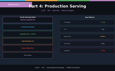
LLM Inference Optimization Part 4 — Production Serving
Production deployment with vLLM and TGI. Continuous Batching, Speculative Decoding, memory budget design, and throughput benchmarks.
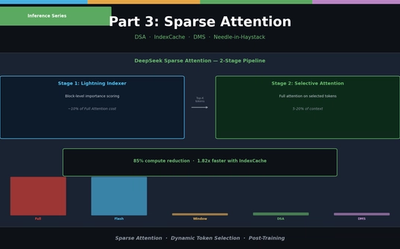
LLM Inference Optimization Part 3 — Sparse Attention in Practice
Sliding Window, Sink Attention, DeepSeek DSA, IndexCache, and Nvidia DMS. From dynamic token selection to Needle-in-a-Haystack evaluation.
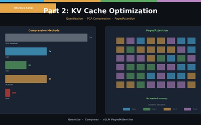
LLM Inference Optimization Part 2 — KV Cache Optimization
KV Cache quantization (int8/int4), PCA compression (KVTC), and PagedAttention (vLLM). Hands-on memory reduction code and scenario-based configuration guide.