Inside Karpathy's autoresearch — Building an AI Research Lab in 630 Lines
A code-level deep dive into Karpathy's autoresearch. Dissecting train.py, BPE tokenizer, MuonAdamW optimizer, and the agent protocol design.

Inside Karpathy's autoresearch -- Building an AI Research Lab in 630 Lines
Andrej Karpathy released autoresearch in March 2026. This post is a code-level deep dive into how a single 630-line train.py lets an AI agent autonomously run 100+ ML experiments overnight.
This is Part 1 of a 3-part series on autoresearch.
- [Part 1](/post/autoresearch-part1-en) (this post): Project structure and deep code analysis
- [Part 2](/post/autoresearch-part2-en): Running it yourself and analyzing the results
- [Part 3](/post/autoresearch-part3-en): Adapting autoresearch to your own domain
1. "Research While You Sleep"
Karpathy opens the README with this vision of the future:
*One day, frontier AI research used to be done by meat computers in between eating, sleeping, having other fun, and synchronizing once in a while using sound wave interconnect in the ritual of "group meeting". That era is long gone. Research is now entirely the domain of autonomous swarms of AI agents running across compute cluster megastructures in the skies. The agents claim that we are now in the 10,205th generation of the code base, in any case no one could tell if that's right or wrong as the "code" is now a self-modifying binary that has grown beyond human comprehension. This repo is the story of how it all began.*
Half joke, half prophecy -- but the direction autoresearch points toward is clear.
Here's the one-line summary: Give an AI agent a small but real LLM training setup, and let it autonomously iterate on experiments overnight.
The agent modifies code, trains for 5 minutes, keeps improvements, reverts failures, and repeats. While you sleep for 8 hours, roughly 100 experiments get run.
2. Project Structure -- Just 3 Files
prepare.py      -- Data + tokenizer + dataloader + evaluation (read-only)
train.py        -- GPT model + optimizer + training loop (agent modifies this)
program.md      -- Agent instructions (human edits this)
pyproject.toml  -- Dependency management
Each file has a sharply defined role:
| File | Lines | Modified by | Role |
|---|---|---|---|
prepare.py | 389 | Nobody (frozen) | Data download, BPE tokenizer, dataloader, evaluate_bpb |
train.py | 631 | AI agent | GPT architecture, MuonAdamW optimizer, training loop |
program.md | 114 | Human | Agent behavior protocol, experiment loop rules |
pyproject.toml | 27 | Nobody (frozen) | PyTorch 2.9.1, kernels, rustbpe, and other dependencies |
The core design principle: The agent only touches `train.py`. The evaluation criteria (`prepare.py`) never change. Humans only edit `program.md`.
We'll come back to why this separation matters.
3. Deep Dive into prepare.py -- The Foundation of Every Experiment
prepare.py is the file the agent can never modify. The rules and evaluation criteria for all experiments are locked in here.
3.1 Constants -- The Rules of the Game
MAX_SEQ_LEN = 2048       # Context length
TIME_BUDGET = 300        # Training time budget: 5 minutes (seconds)
EVAL_TOKENS = 40 * 524288  # Validation tokens: ~20.97 million tokens
The 5-minute time limit is central to autoresearch's design. Whether the agent scales up the model, changes the batch size, or flips the architecture upside down -- only the results within that fixed time window matter. Since it's wall clock time (not step count), every choice the agent makes gets a fair comparison.
3.2 Data -- climbmix-400b
BASE_URL = "https://huggingface.co/datasets/karpathy/climbmix-400b-shuffle/resolve/main"
MAX_SHARD = 6542        # 6542 total shards
VAL_SHARD = MAX_SHARD   # Last shard fixed for validation
Parquet files are downloaded from the climbmix-400b-shuffle dataset on HuggingFace. The default config downloads only 10 shards, with the last shard (shard_06542) always reserved for validation.
3.3 Tokenizer -- rustbpe
VOCAB_SIZE = 8192
SPLIT_PATTERN = r"""'(?i:[sdmt]|ll|ve|re)|[^\r\n\p{L}\p{N}]?+\p{L}+|\p{N}{1,2}| ?[^\s\p{L}\p{N}]++[\r\n]*|\s*[\r\n]|\s+(?!\S)|\s+"""
This uses the GPT-4 split pattern, but with number tokens limited to {1,2} digits instead of {1,3}. Training happens fast via rustbpe (a Rust-based BPE implementation), then gets converted to tiktoken encoding for storage. The 8192 vocab size is deliberately small for efficient experimentation at this scale.
3.4 Dataloader -- BOS-aligned Packing
The dataloader in this project looks simple but is actually quite sophisticated.
def make_dataloader(tokenizer, B, T, split, buffer_size=1000):
    """
    BOS-aligned dataloader with best-fit packing.
    Every row starts with BOS. Documents packed using best-fit to minimize cropping.
    When no document fits remaining space, crops shortest doc to fill exactly.
    100% utilization (no padding).
    """
Key features:
- BOS-aligned: Every row starts with a BOS (Begin of Sequence) token
- Best-fit packing: Fits the largest document into remaining space to minimize waste
- 100% utilization: No padding tokens. If space remains, the shortest document gets cropped to fill it exactly
- GPU optimization: pin_memory + non_blocking copy for efficient CPU-GPU transfer
Since this dataloader is locked inside prepare.py, the agent can't cheat by tampering with data processing.
3.5 evaluate_bpb -- The One Metric That Rules Them All
@torch.no_grad()
def evaluate_bpb(model, tokenizer, batch_size):
    """
    Bits per byte (BPB): vocab size-independent evaluation metric.
    """
    token_bytes = get_token_bytes(device="cuda")
    val_loader = make_dataloader(tokenizer, batch_size, MAX_SEQ_LEN, "val")
    steps = EVAL_TOKENS // (batch_size * MAX_SEQ_LEN)
    total_nats = 0.0
    total_bytes = 0
    for _ in range(steps):
        x, y, _ = next(val_loader)
        loss_flat = model(x, y, reduction='none').view(-1)
        y_flat = y.view(-1)
        nbytes = token_bytes[y_flat]
        mask = nbytes > 0
        total_nats += (loss_flat * mask).sum().item()
        total_bytes += nbytes.sum().item()
    return total_nats / (math.log(2) * total_bytes)
Why bits per byte (BPB) instead of standard cross-entropy loss?
Regular loss depends on vocab size. A larger vocab means higher per-token loss; a smaller vocab means lower loss. The agent can't change vocab size (since prepare.py is frozen), but BPB provides a principled, fairer comparison metric.
Here's how BPB is calculated:
- Sum the cross-entropy loss for each token in nats
- Sum the UTF-8 byte count of each target token in the original text
- Exclude special tokens (byte count = 0) from both sums
total nats / (ln(2) * total bytes)= bits per byte
Lower is better. Since this function is locked in prepare.py, every experiment the agent runs gets judged by the same standard.
4. Anatomy of train.py -- GPT + Muon in 631 Lines
train.py is the one and only file the agent can freely modify. Model definition, optimizer, and training loop -- all in a single file.
4.1 GPT Architecture
Default Config
@dataclass
class GPTConfig:
    sequence_len: int = 2048
    vocab_size: int = 32768
    n_layer: int = 12
    n_head: int = 6
    n_kv_head: int = 6
    n_embd: int = 768
    window_pattern: str = "SSSL"
These are just the defaults -- the actual config gets overridden in the hyperparameter section.
ASPECT_RATIO = 64       # model_dim = depth * ASPECT_RATIO
HEAD_DIM = 128
DEPTH = 8               # Number of transformer layers
The build_model_config function builds the real config from these values. With DEPTH=8, base_dim = 8 * 64 = 512, which aligns to HEAD_DIM=128 giving n_embd=512 and n_head=4.
CausalSelfAttention -- Flash Attention 3 + Sliding Window
class CausalSelfAttention(nn.Module):
    def __init__(self, config, layer_idx):
        super().__init__()
        # ... (Q, K, V projections)
        self.ve_gate = nn.Linear(self.ve_gate_channels, self.n_kv_head, bias=False) \
            if has_ve(layer_idx, config.n_layer) else None

    def forward(self, x, ve, cos_sin, window_size):
        # ... Q, K, V computation
        # Value residual (ResFormer): input-dependent gate mixes value embedding
        if ve is not None:
            ve = ve.view(B, T, self.n_kv_head, self.head_dim)
            gate = 2 * torch.sigmoid(self.ve_gate(x[..., :self.ve_gate_channels]))
            v = v + gate.unsqueeze(-1) * ve

        cos, sin = cos_sin
        q, k = apply_rotary_emb(q, cos, sin), apply_rotary_emb(k, cos, sin)
        q, k = norm(q), norm(k)  # QK-Norm

        y = fa3.flash_attn_func(q, k, v, causal=True, window_size=window_size)
Three things stand out here.
First, Value Embedding (ResFormer). On alternating layers (has_ve), the input token embeddings are added directly to the values. The gate uses 2 * sigmoid(...), giving a range of [0, 2]. Since the weights are initialized to zero, sigmoid(0) = 0.5, so 2 * 0.5 = 1.0 at initialization. Each layer learns how much to incorporate the value embedding during training.
Second, QK-Norm. After applying RoPE, both Q and K get RMS normalization. This stabilizes the scale of attention logits.
Third, Sliding Window. The SSSL pattern repeats short-short-short-long. Short windows are sequence_len // 2 = 1024, long windows are 2048 (full context). The final layer is always long. This way, most layers only attend to half the context (saving compute), while the last layer synthesizes the full picture.
MLP -- ReLU Squared
class MLP(nn.Module):
    def forward(self, x):
        x = self.c_fc(x)
        x = F.relu(x).square()  # ReLU^2
        x = self.c_proj(x)
        return x
The activation function here is -- not GeLU, not SwiGLU. F.relu(x).square() squares the ReLU output, maintaining sparsity while producing sharper activation patterns. It's simple to implement and computationally lightweight.
Block -- x0 Skip Connection
class Block(nn.Module):
    def forward(self, x, ve, cos_sin, window_size):
        x = x + self.attn(norm(x), ve, cos_sin, window_size)
        x = x + self.mlp(norm(x))
        return x
The Block itself is standard Pre-Norm (RMS Norm) + residual connection. But GPT's forward method adds something special:
def forward(self, idx, targets=None, reduction='mean'):
    x = self.transformer.wte(idx)
    x = norm(x)
    x0 = x  # Save initial embedding
    for i, block in enumerate(self.transformer.h):
        x = self.resid_lambdas[i] * x + self.x0_lambdas[i] * x0  # The key line
        ve = self.value_embeds[str(i)](idx) if str(i) in self.value_embeds else None
        x = block(x, ve, cos_sin, self.window_sizes[i])
    x = norm(x)
Before entering each block, it computes resid_lambdas[i] * x + x0_lambdas[i] * x0. resid_lambdas are initialized to 1.0 and x0_lambdas to 0.1. In other words, every layer mixes in 10% of the initial embedding. This improves gradient flow in deep networks.
Logit Soft-Capping
softcap = 15
logits = self.lm_head(x)
logits = logits.float()
logits = softcap * torch.tanh(logits / softcap)
Logits are smoothly clamped to the range. tanh(z/15) * 15 is nearly an identity function for small and saturates at 15 for large values. This technique, introduced in Gemma 2, significantly improves training stability.
4.2 MuonAdamW Optimizer
The optimizer in train.py isn't plain AdamW. It uses two different optimizers depending on the parameter type:
| Parameter type | Optimizer | Learning rate |
|---|---|---|
lm_head (unembedding) | AdamW | 0.004 |
wte (token embedding) | AdamW | 0.6 |
value_embeds | AdamW | 0.6 |
resid_lambdas | AdamW | 0.005 (0.5 * 0.01) |
x0_lambdas | AdamW | 0.5 |
| Transformer matrices (2D) | Muon | 0.04 |
All AdamW learning rates are scaled by .
The Heart of Muon: Polar Express Orthogonalization
Muon (MomentUm Orthogonalized update) is built around a core idea: push the gradient matrix toward orthogonality. It does this via Newton-Schulz iteration.
polar_express_coeffs = [
    (8.156554524902461, -22.48329292557795, 15.878769915207462),
    (4.042929935166739, -2.808917465908714, 0.5000178451051316),
    # ... 5 sets
]

# Polar express orthogonalization
X = g.bfloat16()
X = X / (X.norm(dim=(-2, -1), keepdim=True) * 1.02 + 1e-6)
if g.size(-2) > g.size(-1):
    for a, b, c in polar_express_coeffs[:ns_steps]:
        A = X.mT @ X
        B = b * A + c * (A @ A)
        X = a * X + X @ B
else:
    for a, b, c in polar_express_coeffs[:ns_steps]:
        A = X @ X.mT
        B = b * A + c * (A @ A)
        X = a * X + B @ X
Five iterations approximate the orthogonal component from the polar decomposition of the gradient matrix. Why does this help? Orthogonal updates improve the condition number of the parameter matrix and stabilize training.
Depending on the matrix's aspect ratio, it chooses whichever of or is smaller -- purely for computational efficiency.
NorMuon -- Variance Reduction
After Polar Express orthogonalization, a variance reduction technique called NorMuon is applied.
# NorMuon variance reduction
v_mean = g.float().square().mean(dim=red_dim, keepdim=True)
second_momentum_buffer.lerp_(v_mean.to(dtype=second_momentum_buffer.dtype), 1 - beta2)
step_size = second_momentum_buffer.clamp_min(1e-10).rsqrt()
This tracks the second moment of gradients per dimension and uses it to normalize step sizes. The effect is that gradient variance across dimensions gets equalized.
Cautious Weight Decay
mask = (g * stacked_params) >= 0
stacked_params.sub_(lr * g + lr * wd * stacked_params * mask)
Standard weight decay applies uniformly to all parameters. Here, decay is only applied when the gradient and parameter have the same sign. The intuition: if the gradient is already pushing a parameter toward zero, the decay is redundant.
4.3 Training Loop Design
Time-Based Training
while True:
    # ... gradient accumulation ...
    progress = min(total_training_time / TIME_BUDGET, 1.0)
    # ... optimizer step ...

    if step > 10 and total_training_time >= TIME_BUDGET:
        break
Training is driven by wall clock time, not step count. The first 10 steps are treated as warmup (including torch.compile compilation) and excluded from timing. After that, total_training_time accumulates until it hits 5 minutes.
Gradient Accumulation
TOTAL_BATCH_SIZE = 2**19  # ~524K tokens
DEVICE_BATCH_SIZE = 128
# tokens_per_fwdbwd = 128 * 2048 = 262,144
# grad_accum_steps = 524,288 / 262,144 = 2
Each optimizer step uses about 524K tokens. Due to GPU memory constraints, this is split across 2 forward-backward passes.
LR Schedule
WARMUP_RATIO = 0.0      # No warmup
WARMDOWN_RATIO = 0.5    # Cosine decay in the last 50%
FINAL_LR_FRAC = 0.0     # Final LR = 0

def get_lr_multiplier(progress):
    if progress < WARMUP_RATIO:
        return progress / WARMUP_RATIO if WARMUP_RATIO > 0 else 1.0
    elif progress < 1.0 - WARMDOWN_RATIO:
        return 1.0
    else:
        cooldown = (1.0 - progress) / WARMDOWN_RATIO
        return cooldown * 1.0 + (1 - cooldown) * FINAL_LR_FRAC
No warmup. The first 50% runs at full learning rate, then linearly decays to 0 over the remaining 50%. With only 5 minutes of training, spending time on warmup is a waste.
Muon's momentum also has its own schedule:
def get_muon_momentum(step):
    frac = min(step / 300, 1)
    return (1 - frac) * 0.85 + frac * 0.95
It starts at 0.85 and ramps up to 0.95 over 300 steps.
GC Management -- Preventing 500ms Stalls
if step == 0:
    gc.collect()
    gc.freeze()
    gc.disable()
elif (step + 1) % 5000 == 0:
    gc.collect()
Python's garbage collector can fire without warning and cause up to 500ms stalls. In a 5-minute training run, that's devastating. So after the first step, all objects get collected, gc.freeze() promotes them to the permanent generation, and gc.disable() turns off automatic GC entirely.
Fail Fast
train_loss_f = train_loss.item()
if math.isnan(train_loss_f) or train_loss_f > 100:
    print("FAIL")
    exit(1)
If the loss is NaN or exceeds 100, training terminates immediately. This is a safety valve so the agent doesn't waste the full 5 minutes on a reckless experiment.
5. program.md -- The Agent's Research Protocol
program.md is a 114-line Markdown file, but it's the brain of autoresearch. Karpathy calls it the "research org code."
Setup Phase
Here's the procedure when the agent first starts:
- Agree on a run tag: Suggest a date-based tag (e.g.,
mar5) - Create a branch:
git checkout -b autoresearch/<tag> - Read files: Read README.md, prepare.py, train.py in full
- Check data: Verify
~/.cache/autoresearch/exists - Initialize results.tsv: Create a TSV file with headers only
Experiment Loop -- LOOP FOREVER
LOOP FOREVER:
1. Check git status
2. Modify train.py (experimental idea)
3. git commit
4. uv run train.py > run.log 2>&1
5. Extract results: grep "^val_bpb:\|^peak_vram_mb:" run.log
6. On crash, check stack trace: tail -n 50
7. Record in results.tsv
8. If improved, keep; otherwise git reset
All of the agent's output is redirected to run.log. No tee is used -- this is intentional, so training logs don't eat up the agent's context window.
Results are recorded in TSV (tab-separated) format:
commit	val_bpb	memory_gb	status	description
a1b2c3d	0.997900	44.0	keep	baseline
b2c3d4e	0.993200	44.2	keep	increase LR to 0.04
c3d4e5f	1.005000	44.0	discard	switch to GeLU activation
d4e5f6g	0.000000	0.0	crash	double model width (OOM)
The Cardinal Rule: "NEVER STOP"
This is the most important sentence in program.md:
NEVER STOP: Once the experiment loop has begun, do NOT pause to ask the human if you should continue. Do NOT ask "should I keep going?" or "is this a good stopping point?". The human might be asleep, or gone from a computer and expects you to continue working *indefinitely* until you are manually stopped.
If the agent asks "should I continue?" while the human is sleeping, 8 hours are wasted. When ideas run dry, the instructions say to re-read the code, reference papers, and recombine previous failures.
Simplicity Bar
A 0.001 val_bpb improvement that adds 20 lines of hacky code? Probably not worth it.
A 0.001 val_bpb improvement from deleting code? Definitely keep.
An improvement of ~0 but much simpler code? Keep.
This is pure Karpathy. Complexity-increasing improvements need to earn their keep, while achieving the same performance with less code is always a win.
VRAM Is a Soft Constraint
VRAM is a soft constraint. Some increase is acceptable for meaningful val_bpb gains, but it should not blow up dramatically.
Memory usage is tracked but not strictly limited. If a change causes OOM, it naturally gets discarded as a crash.
6. Real Results -- 100 Experiments Overnight
Karpathy's Official Results
When Karpathy released this project, he also shared his own experimental results. The results on a single H100 GPU were impressive: the agent (Claude) iterated overnight and cut GPT-2 training time from 2.02 hours to 1.80 hours -- an ~11% reduction.
Some interesting discoveries the agent made:
- Fixed a bug related to attention scaling
- Identified a missing regularization issue
- Found subtle optimizations that even a 20-year veteran researcher might miss
Shopify CEO's Experiment
Shopify CEO Tobi Lutke also forked autoresearch and ran his own experiments. His runs showed a 19% improvement in val_bpb. Interestingly, the agent found a smaller model that outperformed the original larger one. Within the 5-minute constraint, finding an efficient architecture matters more than blindly scaling up -- and the agent figured that out on its own.
Community Spread
Forks proliferated across platforms almost immediately after release:
| Fork | Platform |
|---|---|
| miolini/autoresearch-macos | macOS |
| trevin-creator/autoresearch-mlx | macOS (MLX) |
| jsegov/autoresearch-win-rtx | Windows RTX |
Karpathy also provides a tuning guide in the README for smaller compute setups, recommending the TinyStories dataset, reduced vocab size, lower MAX_SEQ_LEN, and fewer DEPTH layers.
7. Why This Matters -- A Paradigm Shift in AI Research
Automating Research
The traditional ML research loop looks like this:
Human: form hypothesis -> write code -> run experiment -> analyze results -> repeatautoresearch transforms it into:
Agent: generate idea -> modify train.py -> train 5 min -> check val_bpb -> keep/discard -> repeatThe entire loop -- from hypothesis to evaluation -- has been handed to the agent.
Core Insight: Two Editing Layers
The most elegant design in autoresearch is the separation of what gets edited:
Human  -> edits program.md   (research strategy, agent behavior rules)
Agent  -> edits train.py     (model architecture, hyperparameters)
Humans code the "what direction to research," while the agent executes "what specific code to write." program.md is "meta-code" that governs the agent's behavior.
The Meta-optimization Possibility
Take this one step further and you can imagine an outer loop that optimizes program.md itself:
Outer agent: modify program.md -> inner agent runs 100 experiments -> evaluate program.md by final val_bpbThis would be automatically optimizing the structure of the research organization itself. Karpathy directly mentions this possibility in the README: "how you'd iterate on it over time to find the 'research org code' that achieves the fastest research progress."
Limitations
The current autoresearch has clear limitations:
- Single GPU: No distributed training
- Single file: Only
train.pycan be modified - 5-minute experiments: Long-duration training runs aren't possible
- Numeric metric only: Judged solely by val_bpb (generation quality, reasoning ability, etc. are not captured)
- Search scope: Depends on the agent's creativity (no structured exploration strategy)
These constraints are exactly why Karpathy himself calls it "the story of how it all began." It's just the beginning, but the direction is compelling.
8. What's Next
This post covered autoresearch's structure and code.
- [Part 2](/post/autoresearch-part2-en) walks through running autoresearch yourself and analyzing the experiments the agent produces overnight. We'll look at which ideas succeed, which fail, and the patterns in the agent's research behavior.
- [Part 3](/post/autoresearch-part3-en) covers adapting autoresearch to your own domain -- how to customize program.md, how to modify prepare.py for different tasks, and practical strategies for using this in production settings.
*The code analyzed in this post is from the karpathy/autoresearch repository as of March 2026.*
Part 1 of 4 complete
3 more parts waiting for you
From theory to production deployment — subscribe to unlock the full series and all premium content.
Subscribe to Newsletter
Related Posts
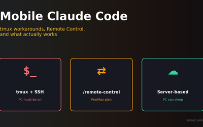
Mobile Claude Code: three approaches, and what actually works
Three ways to reach Claude Code from your phone — tmux + SSH, /remote-control, and server-based agents. The real fix isn't "mobile support" but decoupling compute from your device.

Inside Google COSMO — The New Architecture of On-Device AI Agents
Deep-dive into COSMO, Google's next-gen AI assistant accidentally leaked before I/O 2026. Full breakdown of the 3-mode architecture: Gemini Nano + PI server + Hybrid routing.

Self-Evolving AI Agents — The New Paradigm of 2026
GenericAgent, Evolver, Open Agents — comparing 3 self-evolving agent frameworks that learn, adapt, and grow without human coding.