The Transformer Block from 2017 to Mamba Hybrids: 15 Changes, 13 Rebuilt in Code
Fifteen changes to the Transformer block, from Post-LN to Mamba hybrids, each drawn as one diagram and explained with what the paper reported and what it costs. We rebuilt one layer from seven real models as short PyTorch functions; all seven match the Hugging Face output. On the same sentence, the residual stream grows 98-fold from the first layer to the last in Qwen3-0.6B and only 1.1-fold in BERT.
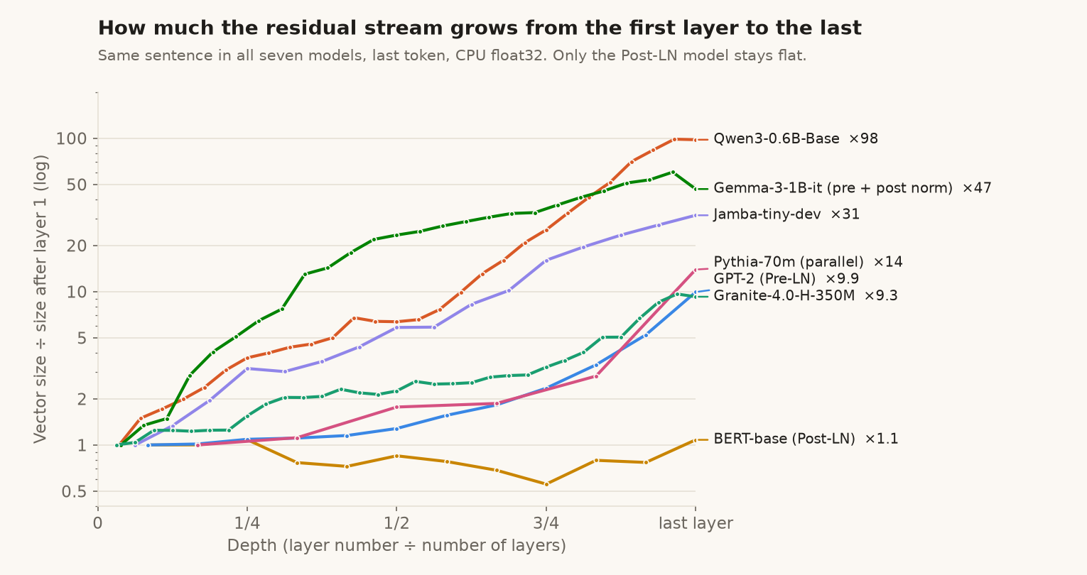
We fed one sentence to seven models, BERT, GPT-2, Pythia, Qwen3, Gemma 3, Jamba and Granite-4.0-H, and measured how large the last token's vector gets after each layer. In Qwen3-0.6B-Base it ends 98 times larger than after the first layer. In BERT it ends 1.1 times larger, almost the same. Both are built from the same three cells, attention, a feed-forward network and a norm, though they differ in many other ways too. One difference shows up directly in this chart: BERT renormalizes the residual stream itself after every addition, and the other six never normalize it. That is why only BERT's line stays flat. Where the norm sits is one of the fifteen changes this post walks through.
In the previous post we followed one token through GPT-2, Qwen3 and Granite. Every layer had the same steps: normalize, mix information across tokens, add the result back, normalize, transform each token with a feed-forward network (FFN), add back. This post is about how those cells have been filled, wired and stacked since 2017. For each change there is one animated diagram, what the paper reported, and what it costs. The attention calculation itself (heads, KV cache, grouped queries, sparse and linear attention) is covered in the attention roundup, so here attention is a single cell.
How we checked the code
Every block in this post comes with a short PyTorch function. To know that a function is the real block and not our reading of a paper, we compared it with the actual model:
- Load the model from Hugging Face and run the sentence "In the morning, Alice gave Bob a book. Later, Bob gave the book back to" through it.
- While it runs, record what goes into and comes out of each layer. PyTorch calls this a forward hook.
- Take one layer's weights, give our function the same input, and compare its output with what the real layer produced.
io = {}
def hook(i):
    def f(mod, args, kwargs, out):
        x = args[0] if args else kwargs["hidden_states"]   # what went into layer i
        y = out[0] if isinstance(out, tuple) else out       # what came out
        io[i] = (x[0].clone(), y[0].clone())
    return f
hs = [l.register_forward_hook(hook(i), with_kwargs=True) for i, l in enumerate(layers)]
model(ids)

x, y = io[5]                                     # layer 5
ours = pre_ln_block(x, weights_of_layer_5, n_heads, eps)
print((ours - y).abs().max())                    # largest difference over all numbers
We ran this on a CPU in float32 for 22 layers across seven models (the full script is in the repro bundle at the end). The largest difference, divided by the largest value in the real output, was 3.9e-5, in Pythia's last layer. Every other check was 2.2e-7 or less. Pythia's last layer stands out, so we ran the three Pythia checks again in float64: the gap in that layer fell to 5.4e-13, and in the other two to 2.3e-15 or less. A gap that shrinks with the precision is rounding, not a different calculation, so the functions compute the same thing as the models.
| Model | What it checks | Layers compared | Largest relative difference |
|---|---|---|---|
| BERT-base | Post-LN | 0, 5, 11 | 2.2e-7 |
| GPT-2 | Pre-LN | 0, 5, 11 | 1.8e-7 |
| Pythia-70m | parallel block, partial RoPE | 0, 2, 5 | 3.9e-5 |
| Qwen3-0.6B-Base | RMSNorm, QK-norm, RoPE, SwiGLU | 0, 14, 27 | 1.4e-7 |
| Gemma-3-1B-it | norm before and after each cell | 2, 5, 25 | 4.5e-8 |
| Jamba-tiny-dev | Mamba, MoE, attention without positions | 3, 4, 5, 12 | 9.4e-8 |
| Granite-4.0-H-350M | Mamba-2, attention without positions | 0, 10, 31 | 1.6e-7 |
The code shown below is the code that passed these checks. Two items, the encoder-decoder original and Hymba, are explained with diagrams and the papers' numbers.
Where it started
1. The original block (2017)
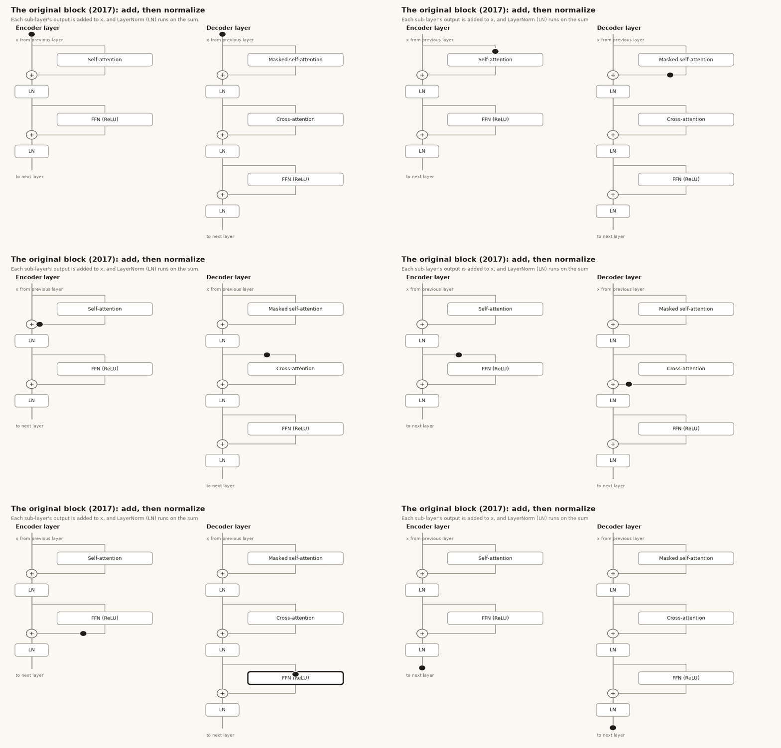
"Attention Is All You Need" (Vaswani et al., 2017) built a translation model from an encoder and a decoder, six layers each. Each sub-layer is wrapped as LayerNorm(x + Sublayer(x)): compute the cell, add its output to x, then normalize the sum. This is called Post-LN, because the norm comes after the addition. The FFN is two matrices with a ReLU between them, 512 wide outside and 2,048 inside. Positions were added to the input as fixed sine waves; the paper also tried learned position vectors and reports the same BLEU, 25.7, for both (Table 3, row E).
BERT kept this block for its encoder (with GELU in the FFN), so BERT-base is our working Post-LN example:
def post_ln_block(x, sd, H, eps):
    q = heads(x @ sd["attention.self.query.weight"].T + sd["attention.self.query.bias"], H)
    k = heads(x @ sd["attention.self.key.weight"].T + sd["attention.self.key.bias"], H)
    v = heads(x @ sd["attention.self.value.weight"].T + sd["attention.self.value.bias"], H)
    a = merge(attend(q, k, v, 1 / math.sqrt(q.shape[-1]), causal=False))
    a = a @ sd["attention.output.dense.weight"].T + sd["attention.output.dense.bias"]
    x = layer_norm(x + a, sd["attention.output.LayerNorm.weight"], sd["attention.output.LayerNorm.bias"], eps)
    f = F.gelu(x @ sd["intermediate.dense.weight"].T + sd["intermediate.dense.bias"])
    f = f @ sd["output.dense.weight"].T + sd["output.dense.bias"]
    return layer_norm(x + f, sd["output.LayerNorm.weight"], sd["output.LayerNorm.bias"], eps)
Look at the two layer_norm(x + ...) lines: the stream x itself is renormalized twice per layer. That is why BERT's line in the first chart stays flat.
2. Decoder only
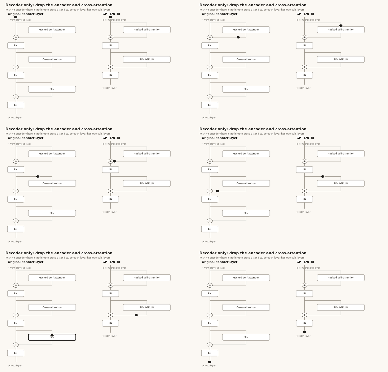
A language model that only continues text has no source sentence to read, so it does not need the encoder or the cross-attention that reads from it. GPT (Radford et al., 2018) stacked 12 decoder layers with masked self-attention and an FFN: 768 wide, 3,072 inside. The same paper switched the FFN activation to GELU and used learned position vectors instead of sine waves. Almost every model below is this decoder-only stack with different cells.
The norm cell
3. Pre-LN: normalize the copy, not the stream
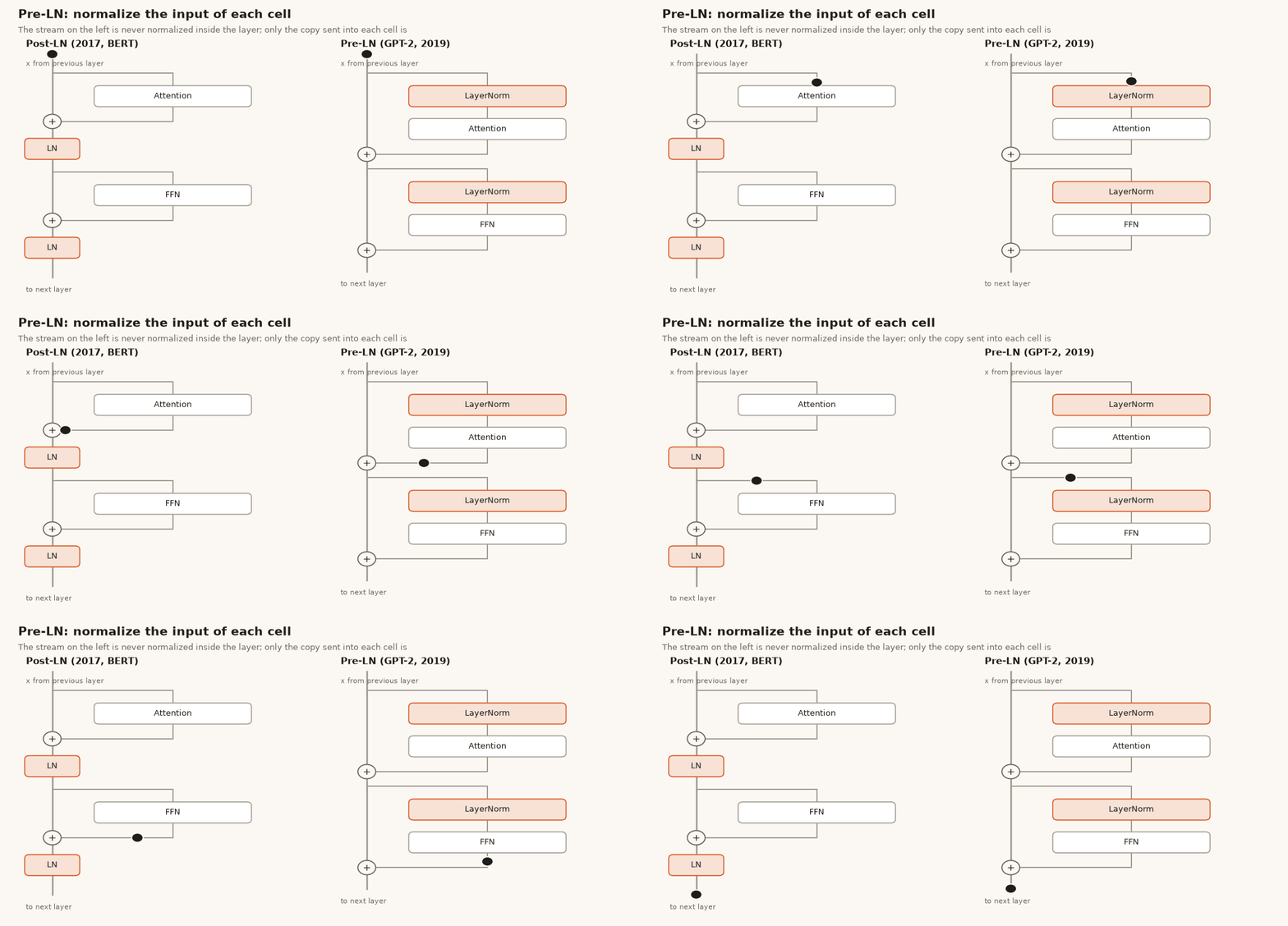
GPT-2 (Radford et al., 2019) states three changes from GPT: LayerNorm "was moved to the input of each sub-block", one more LayerNorm was added after the last block, and residual weights were scaled down by 1/√N at initialization. In code the difference from BERT is where the norm call goes:
def pre_ln_block(x, sd, H, eps):
    D = x.shape[-1]
    h = layer_norm(x, sd["ln_1.weight"], sd["ln_1.bias"], eps)      # normalize a copy
    q, k, v = (heads(t, H) for t in (h @ sd["attn.c_attn.weight"] + sd["attn.c_attn.bias"]).split(D, -1))
    a = merge(attend(q, k, v, 1 / math.sqrt(D // H)))
    x = x + a @ sd["attn.c_proj.weight"] + sd["attn.c_proj.bias"]   # add to the raw stream
    h = layer_norm(x, sd["ln_2.weight"], sd["ln_2.bias"], eps)
    f = F.gelu(h @ sd["mlp.c_fc.weight"] + sd["mlp.c_fc.bias"], approximate="tanh")
    return x + f @ sd["mlp.c_proj.weight"] + sd["mlp.c_proj.bias"]
Why it helps. Xiong et al. (2020) showed that at initialization a Post-LN model has large gradients near the output, so it needs a learning-rate warm-up to train well; on IWSLT14 German-English, Post-LN without warm-up reached only 8.45 BLEU against about 34 with it. Pre-LN gradients are well-behaved, so warm-up can be dropped. In their BERT pre-training run, Pre-LN reached a validation loss of about 1.69 near 500k steps and Post-LN only near 700k (their Figure 5a), which they report as a 40% speed-up.
What it costs. The stream is never normalized inside the stack, so every layer's output accumulates. That is the growth in the first chart: GPT-2's last-token vector goes from 51.6 after layer 1 to 512.1 after layer 12. A final norm before the output (the extra LayerNorm GPT-2 added) handles the scale at the end.
4. RMSNorm: drop the mean
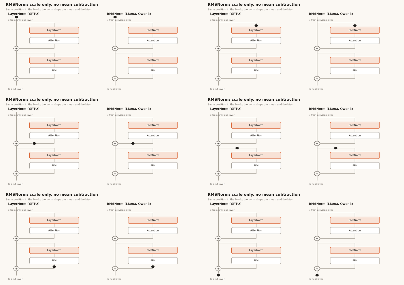
LayerNorm subtracts the mean of the vector, divides by the standard deviation, then multiplies by a weight and adds a bias. RMSNorm (Zhang and Sennrich, 2019) keeps only the scaling: divide by the root mean square and multiply by a weight.
def rms_norm(x, w, eps, plus_one=False):
    y = x * torch.rsqrt(x.pow(2).mean(-1, keepdim=True) + eps)
    return y * (1 + w) if plus_one else y * w           # Gemma multiplies by (1 + w)
What the paper reports. On a Transformer-base translation model the time per 1,000 training steps fell from 248 to 231 seconds, 6.9% (Table 4), with BLEU 26.6 vs 26.8 on newstest2014. The abstract's "7% to 64%" range includes RNN models; for the Transformer the reported gains are 6.9% for RMSNorm and 9% for its partial variant, pRMSNorm. Cost: none stated beyond losing re-centering, which the authors argue is not needed.
5. A norm on both sides of each cell (Gemma 2 and 3)
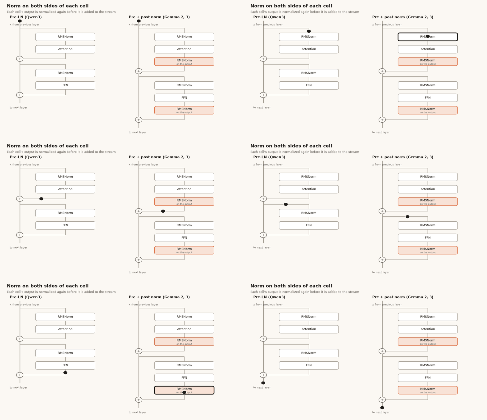
Gemma 2 (Gemma Team, 2024) normalizes "the input and output of each transformer sub-layer"; Gemma 3 (Gemma Team, 2025) keeps it. Each Gemma 3 layer therefore has four norms: input_layernorm, post_attention_layernorm, pre_feedforward_layernorm, post_feedforward_layernorm.
def sandwich_block(x, sd, Hq, Hkv, d, eps, theta, scale):
    pos = torch.arange(x.shape[0])
    n = lambda t, name: rms_norm(t, sd[name], eps, plus_one=True)
    h = n(x, "input_layernorm.weight")
    q = n(heads(h @ sd["self_attn.q_proj.weight"].T, Hq), "self_attn.q_norm.weight")
    k = n(heads(h @ sd["self_attn.k_proj.weight"].T, Hkv), "self_attn.k_norm.weight")
    v = heads(h @ sd["self_attn.v_proj.weight"].T, Hkv)
    q, k = rope(q, pos, theta), rope(k, pos, theta)
    a = merge(attend(q, k, v, scale)) @ sd["self_attn.o_proj.weight"].T
    x = x + n(a, "post_attention_layernorm.weight")                  # norm the output, then add
    h = n(x, "pre_feedforward_layernorm.weight")
    g, u = h @ sd["mlp.gate_proj.weight"].T, h @ sd["mlp.up_proj.weight"].T
    f = (F.gelu(g, approximate="tanh") * u) @ sd["mlp.down_proj.weight"].T
    return x + n(f, "post_feedforward_layernorm.weight")
A naming trap if you read the weights: in Llama and Qwen3, post_attention_layernorm is the norm before the FFN. In Gemma it really is applied to the attention output.
The output norm limits how much each cell can add, but the stream itself is still never normalized, so it still grows: 47-fold in our chart. That is more than GPT-2's 9.9-fold, but the two models differ in size and training too, so the chart cannot isolate the effect of the output norm. What the papers report: the reason given is "to stabilize training"; neither report gives a number for this change. Cost: two more norm calls per layer.
6. QK-norm: normalize queries and keys
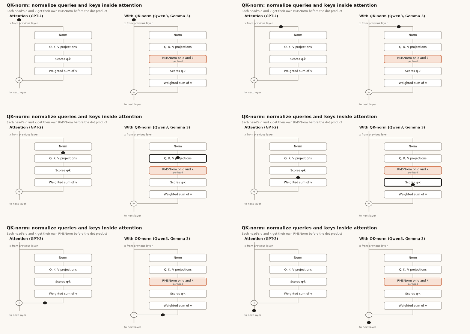
Attention scores are dot products of queries and keys. If those vectors grow during training, the scores grow and softmax puts nearly all weight on one token. ViT-22B (Dehghani et al., 2023) hit exactly this at about 8B parameters: training diverged because attention logits became extremely large. In their runs without the normalization, logits grew "to over 50000 in magnitude". Their fix, which they credit to Gilmer et al. (2023), was a LayerNorm on the queries and keys before the dot product. An earlier paper (Henry et al., 2020) used L2 normalization with a learned scale and reported 0.928 BLEU better on average over five low-resource translation pairs.
Qwen3 (Yang et al., 2025) removed the QKV bias of Qwen2 and added QK-norm "to ensure stable training"; Gemma 3 replaced Gemma 2's logit soft-capping with it. In Qwen3 it is two extra lines, one RMSNorm per head on q and on k:
def qwen3_block(x, sd, Hq, Hkv, d, eps, theta):
    pos = torch.arange(x.shape[0])
    h = rms_norm(x, sd["input_layernorm.weight"], eps)
    q = rms_norm(heads(h @ sd["self_attn.q_proj.weight"].T, Hq), sd["self_attn.q_norm.weight"], eps)
    k = rms_norm(heads(h @ sd["self_attn.k_proj.weight"].T, Hkv), sd["self_attn.k_norm.weight"], eps)
    v = heads(h @ sd["self_attn.v_proj.weight"].T, Hkv)
    q, k = rope(q, pos, theta), rope(k, pos, theta)
    x = x + merge(attend(q, k, v, 1 / math.sqrt(d))) @ sd["self_attn.o_proj.weight"].T
    return x + swiglu(rms_norm(x, sd["post_attention_layernorm.weight"], eps), sd)
This one function also contains items 4, 7 and 10. Cost: a small weight vector per norm (128 numbers each in Qwen3-0.6B) and two norm calls per layer.
The position cell
7. RoPE: position as a rotation inside attention
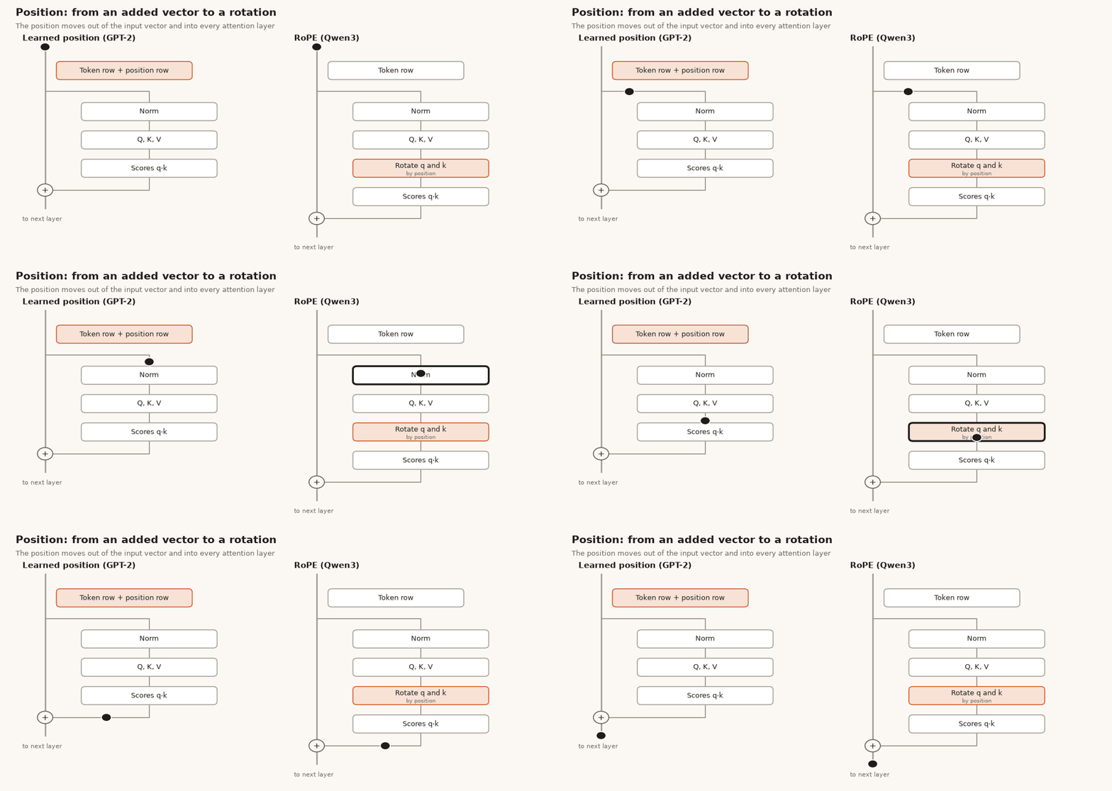
GPT-1 and GPT-2 add a learned position vector to each token vector once, at the bottom; GPT-2 has 1,024 such rows and cannot take a longer input. RoPE (Su et al., 2021) instead rotates pairs of numbers in q and k by an angle proportional to the position, inside every attention layer. The dot product of two rotated vectors then depends on how far apart the tokens are. The previous post has the rope function and a check of that property.
What the paper reports: 27.5 vs 27.3 BLEU on WMT14 English-German against the Transformer base, and on a Chinese legal-matching task, 68.29% accuracy at 512 tokens and 69.79% at 1,024 against 67.77% for the BERT baseline. Limitation stated by the authors: they lack "thorough explanations on why it converges faster". Pythia applies RoPE to only the first quarter of each head (rot_frac = 0.25 in our parallel_block below); Qwen3-Next does the same in its attention layers.
8. NoPE: no position signal at all
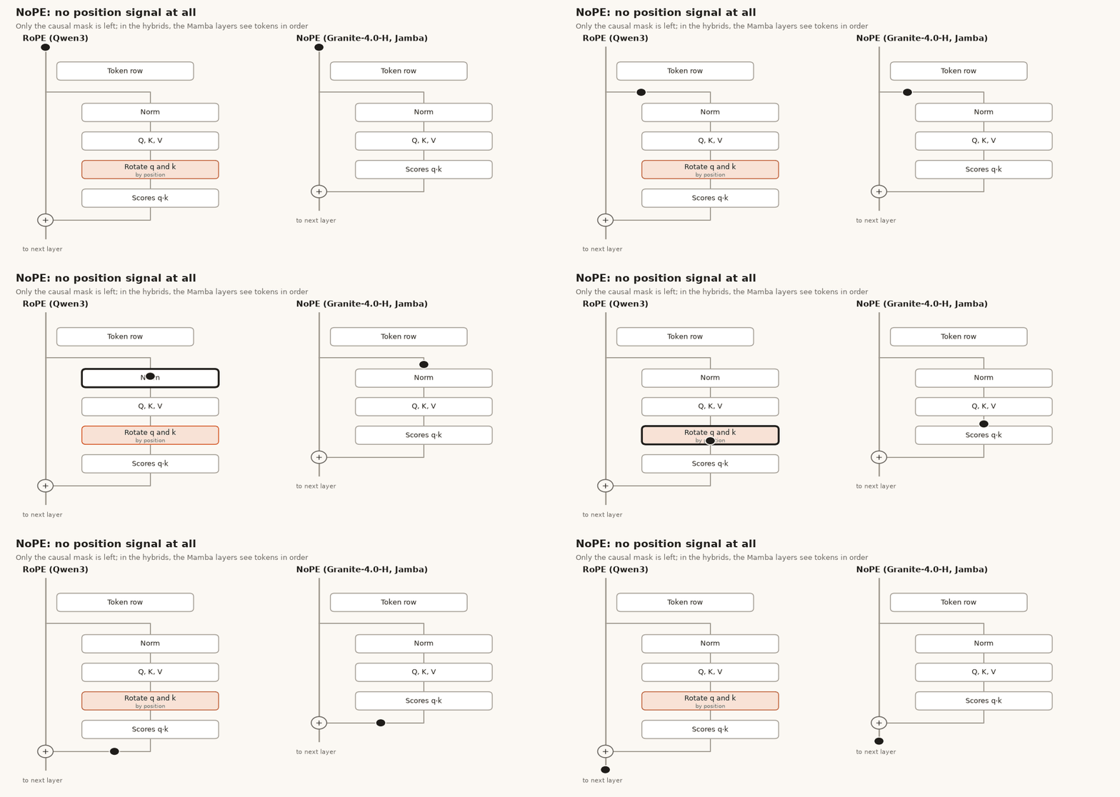
A decoder already has some position information without any encoding: the causal mask lets token 10 see 10 earlier tokens and token 3 see only 3. Kazemnejad et al. (2023) trained small decoder-only models (about 107M parameters) on synthetic reasoning tasks and found that no position encoding generalized to longer inputs better than the explicit methods they tested. Limitation stated: they could not test large-scale pretraining, and in their 1B runs ALiBi was more stable than NoPE at the longest lengths.
The hybrids use NoPE for a different reason. Jamba (Lieber et al., 2024): "with the Mamba layer, positional embeddings or mechanisms like RoPE are not necessary". Granite-4.0-H-350M's config says "position_embedding_type": "nope". A Mamba layer reads tokens in order, so the order is already in its state. Our Jamba and Granite attention code has no rope call, and both matched the real layers.
The wiring
9. Parallel block: attention and FFN read the same input
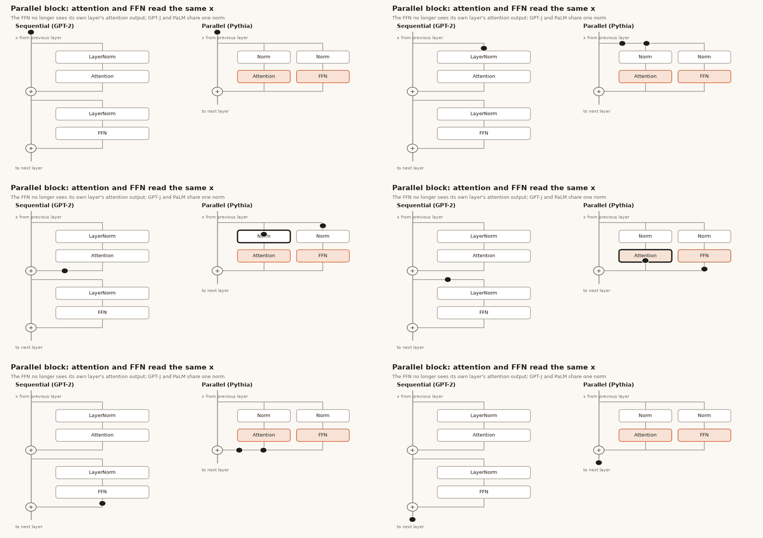
In a normal block the FFN sees x after attention has been added. GPT-J (Wang and Komatsuzaki, 2021) computed both from the same x and added them together. PaLM (Chowdhery et al., 2022) adopted it and reported "roughly 15% faster training speed at large scales, since the MLP and Attention input matrix multiplications can be fused", along with "a small quality degradation at 8B scale but no quality degradation at 62B scale", from which they extrapolated that it would be neutral at 540B. GPT-NeoX and Pythia use it too:
def parallel_block(x, sd, H, eps, theta, rot_frac):
    T, D = x.shape
    pos = torch.arange(T)
    h = layer_norm(x, sd["input_layernorm.weight"], sd["input_layernorm.bias"], eps)
    qkv = (h @ sd["attention.query_key_value.weight"].T + sd["attention.query_key_value.bias"])
    qkv = qkv.view(T, H, 3 * (D // H)).transpose(0, 1)              # [q|k|v] per head
    q, k, v = qkv.chunk(3, -1)
    rd = int((D // H) * rot_frac)                                   # Pythia rotates 1/4 of each head
    q, k = rope(q, pos, theta, rd), rope(k, pos, theta, rd)
    a = merge(attend(q, k, v, 1 / math.sqrt(D // H)))
    a = a @ sd["attention.dense.weight"].T + sd["attention.dense.bias"]
    h2 = layer_norm(x, sd["post_attention_layernorm.weight"], sd["post_attention_layernorm.bias"], eps)
    f = F.gelu(h2 @ sd["mlp.dense_h_to_4h.weight"].T + sd["mlp.dense_h_to_4h.bias"])
    f = f @ sd["mlp.dense_4h_to_h.weight"].T + sd["mlp.dense_4h_to_h.bias"]
    return x + a + f                                                # one addition for both
Pythia has two separate norms (h and h2), not one shared norm. The GPT-NeoX paper (Black et al., 2022) says this was unintentional and that small-scale experiments showed no difference. Cost: inside one layer, the FFN can no longer use what attention just found.
The FFN cell
10. SwiGLU: a gated FFN
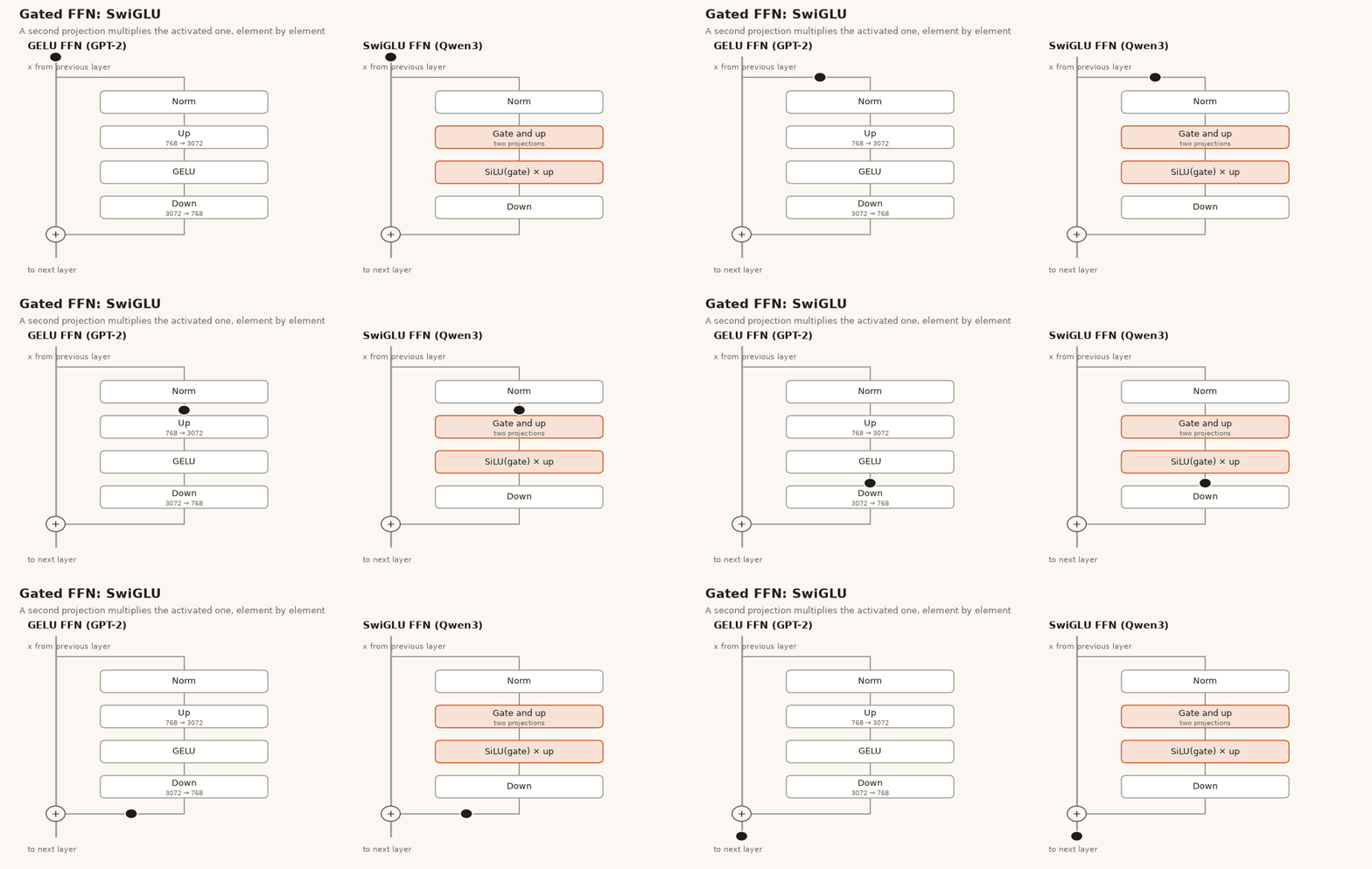
The FFN in GPT-2 is up-project, GELU, down-project. A gated FFN (Shazeer, 2020) adds a second up-projection and multiplies it, element by element, with the activated first one:
def swiglu(h, sd, pre="mlp."):
    return (F.silu(h @ sd[pre + "gate_proj.weight"].T) * (h @ sd[pre + "up_proj.weight"].T)) @ sd[pre + "down_proj.weight"].T
What the paper reports. With parameters and compute matched (the inner width shrinks to 2/3, from 3,072 to 2,048, to pay for the third matrix), held-out log-perplexity on T5-style span filling after 524,288 steps was 1.677 with ReLU, 1.679 with GELU, 1.636 with SwiGLU and 1.633 with GEGLU (lower is better). The author's explanation in full: "We offer no explanation as to why these architectures seem to work; we attribute their success, as all else, to divine benevolence." Qwen3 uses SwiGLU, Gemma uses the GELU version (GeGLU, in sandwich_block above).
11. Mixture of experts: a router picks a few FFNs
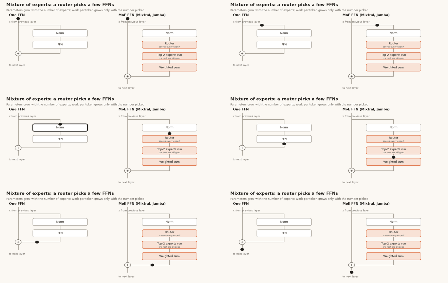
A mixture-of-experts (MoE) layer replaces the single FFN with many FFNs, the experts, and a small router that picks a few for each token. Shazeer et al. (2017) put it between LSTM layers; Switch Transformers (Fedus et al., 2021) put it in place of the Transformer FFN with one expert per token and reported "up to 7x increases in pre-training speed with the same computational resources". Mixtral (Jiang et al., 2024) uses 8 experts and picks 2: 47B parameters in total, 13B used per token.
def moe_ffn(h, sd, top_k):
    p = (h @ sd["feed_forward.router.weight"].T).softmax(-1)        # (tokens, experts)
    w, idx = p.topk(top_k, -1)                                       # Jamba does not renormalize w
    out = torch.zeros_like(h)
    gu, down = sd["feed_forward.experts.gate_up_proj"], sd["feed_forward.experts.down_proj"]
    for t in range(h.shape[0]):
        for j in range(top_k):
            e = idx[t, j]
            g, u = (h[t] @ gu[e].T).chunk(2, -1)
            out[t] += w[t, j] * ((F.silu(g) * u) @ down[e].T)
    return out, idx
Since our function returns which experts it picked, we can look at the routing directly. In Jamba-tiny-dev, 8 experts with 2 per token, layer 3 sends ten of the 19 tokens to expert 0 and only one to expert 4. Layer 5 spreads the same tokens differently, with expert 3 the busiest at nine.
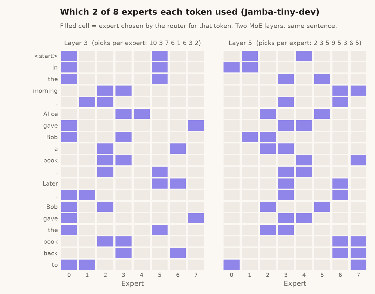
This is one sentence in a small development model, so it shows how routing looks, not which expert does what. Cost stated by Mixtral: memory follows the total parameter count (47B), not the active one, and the routing adds overhead; they call MoE "more suitable for batched workloads". Switch lists "complexity, communication costs and training instability".
Changing the mixing cell
12. Mamba: one cell instead of attention plus FFN
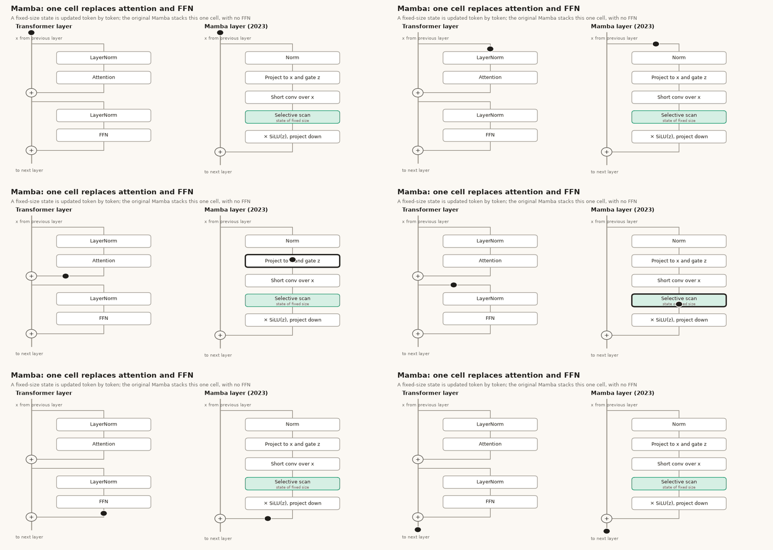
Attention looks back at every earlier token, so the cache grows with the input. Mamba (Gu and Dao, 2023) replaces it with a state of fixed size that is updated once per token. The update depends on the token (that is the "selective" part): a step size dt and the vectors B and C are computed from the input, so the model can decide per token how much to keep and what to write. The original Mamba also drops the FFN: the authors merged the two into one block "stacked homogenously".
This is the sequential version of the scan, from Jamba's Mamba layers:
def mamba1(h, sd, eps):
    T = h.shape[0]
    p = "mamba."
    xs, z = (h @ sd[p + "in_proj.weight"].T).chunk(2, -1)
    w = sd[p + "conv1d.weight"]
    xs = F.conv1d(xs.T[None], w, sd[p + "conv1d.bias"], padding=w.shape[-1] - 1, groups=w.shape[0])[0, :, :T].T
    xs = F.silu(xs)
    N, R = sd[p + "A_log"].shape[1], sd[p + "dt_proj.weight"].shape[1]
    dt, B, C = (xs @ sd[p + "x_proj.weight"].T).split([R, N, N], -1)
    dt, B, C = rms_norm(dt, sd[p + "dt_layernorm.weight"], eps), rms_norm(B, sd[p + "b_layernorm.weight"], eps), rms_norm(C, sd[p + "c_layernorm.weight"], eps)
    dt = F.softplus(dt @ sd[p + "dt_proj.weight"].T + sd[p + "dt_proj.bias"])   # step size per token
    A = -torch.exp(sd[p + "A_log"])                                  # (channels, N)
    state = torch.zeros_like(A)
    ys = []
    for t in range(T):
        state = torch.exp(dt[t][:, None] * A) * state + (dt[t] * xs[t])[:, None] * B[t][None]
        ys.append(state @ C[t] + sd[p + "D"] * xs[t])
    return (torch.stack(ys) * F.silu(z)) @ sd[p + "out_proj.weight"].T
The loop line is the whole idea: shrink the old state by exp(dt * A), write the new input through B, read out through C. (The three rms_norm calls on dt, B and C are Jamba's addition, not part of the original Mamba. Jamba also puts an FFN or MoE cell after each Mamba cell, as jamba_block in the repro bundle does, so its layers are not the FFN-free blocks of the Mamba paper.)
What the paper reports: 4-5 times the inference throughput of a Transformer of similar size, "since without the KV cache it can use much higher batch sizes", and Mamba-3B matching Transformers twice its size. Limitation stated: the evaluation is limited to small models. Jamba's paper adds one: a pure Mamba model "often does not follow the correct format" in few-shot prompts, which they read as weaker in-context learning.
13. Mamba-2: the same scan, simpler and in heads
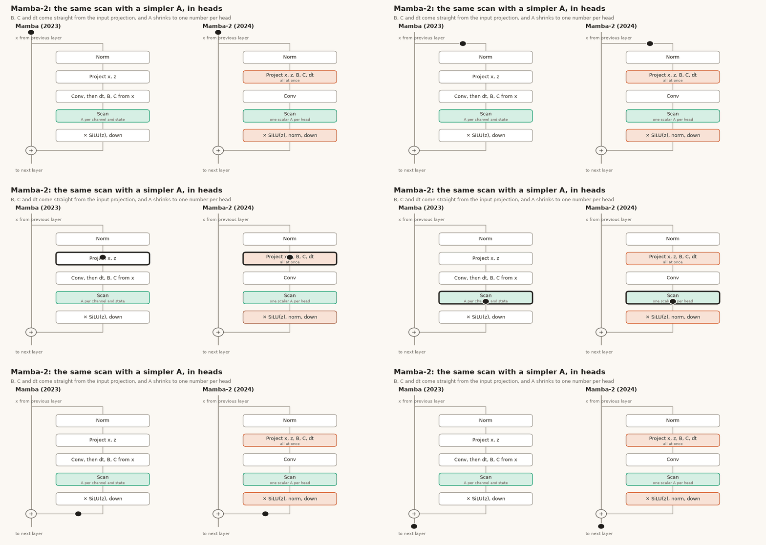
Mamba-2 (Dao and Gu, 2024) makes three changes to the block. B, C and dt come straight from the input projection instead of being computed from x after the convolution. A becomes one number per head instead of a matrix per channel, which lets the scan be computed with matrix multiplications. A norm is added before the output, because "instabilities were prone to arising in larger models". The paper reports the new scan as 2-8 times faster than Mamba's, while allowing a state eight times larger.
Granite-4.0-H uses Mamba-2. Its layers, unlike pure Mamba, keep an FFN after the mixing cell, and scale both additions by 0.246. We verified Granite with the Mamba-2 function from the previous post, which also walks through it:
h = rms_norm(x, sd[p + "input_layernorm.weight"], eps)
mix, _ = mamba2(sd, p, cfg, h)       # in the 4 attention layers: attention with no rope call
x2 = x + mix * cfg.residual_multiplier                                # 0.246
h2 = rms_norm(x2, sd[p + "post_attention_layernorm.weight"], eps)
g, u = (h2 @ sd[p + "shared_mlp.input_linear.weight"].T).chunk(2, -1)
out = x2 + (F.silu(g) * u) @ sd[p + "shared_mlp.output_linear.weight"].T * cfg.residual_multiplier
Stacking
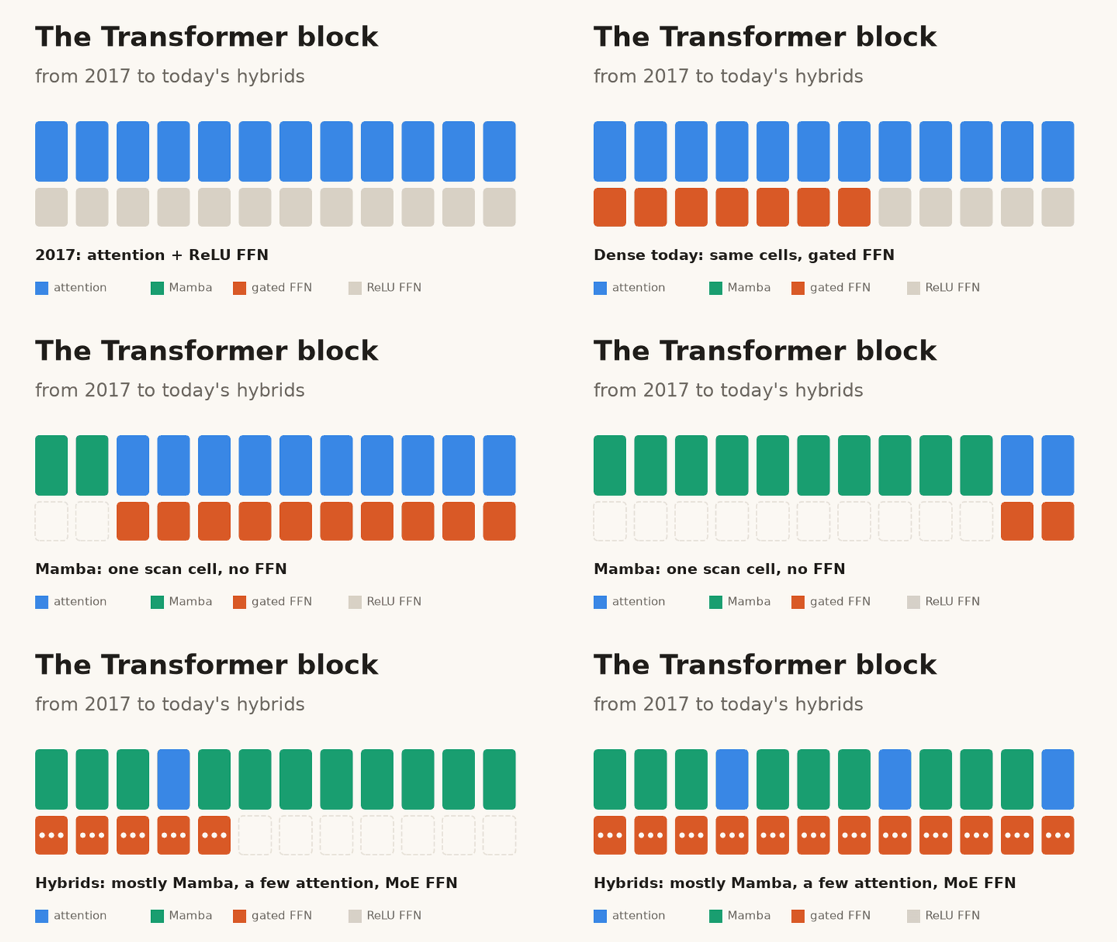
14. Hybrids: mostly Mamba, a few attention layers
The Mamba-2 paper itself tried mixing: at 350M parameters and 48 layers, perplexity on the Pile was 8.60 with no attention layers, 8.26 with six, and 8.68 for a Transformer (Table 2, lower is better), and the authors write that "around 10% of the total number of layers being attention performs best". Jamba compared one attention layer in four with one in eight and found "virtually no performance difference", so they chose one in eight.
Each model's config lists which layer is which, so we drew them straight from the configs:
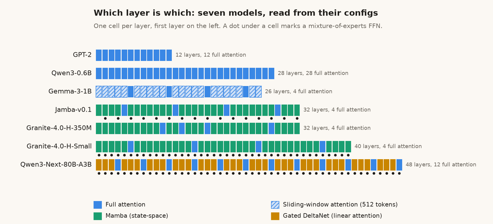
The patterns differ more than the "hybrid" label suggests. Jamba repeats one attention layer every eight. IBM describes Granite-4.0-H Micro, Tiny and Small as Mamba-2 and attention "in a 9:1 ratio"; the small 350M model we ran has 28 Mamba-2 layers and 4 attention layers, and the attention layers sit at uneven positions. Qwen3-Next (model card) does not use Mamba at all: three of every four layers are Gated DeltaNet, a form of linear attention, and every fourth is full attention, with 512 experts per layer and 10 used per token. Gemma 3 is not a hybrid in this sense, but it stacks the same idea within attention: five sliding-window layers that only see the last 512 tokens for every full one.
What it buys. The cache only grows in the full-attention layers. We computed the cache for one sequence at 16 bits from each config (our script adds 2 × KV heads × head size × 2 bytes per token for each full-attention layer, the same capped at 512 tokens for sliding layers, and a fixed state for each Mamba or DeltaNet layer):
| Model | Layers that grow with the input | Per token | Fixed | At 4K tokens | At 128K tokens |
|---|---|---|---|---|---|
| Qwen3-0.6B-Base | 28 of 28 | 112 KiB | 0 | 448 MiB | 14,336 MiB |
| Gemma-3-1B | 4 of 26 (22 capped at 512) | 4 KiB | 0 | 27 MiB | 523 MiB |
| Granite-4.0-H-350M | 4 of 32 | 4 KiB | 10.8 MiB | 27 MiB | 523 MiB |
| Jamba-v0.1 | 4 of 32 | 16 KiB | 8.3 MiB | 72 MiB | 2,056 MiB |
| Qwen3-Next-80B-A3B | 12 of 48 | 24 KiB | 37.7 MiB | 134 MiB | 3,110 MiB |
These are calculated from each model's config at 16 bits, and the models are of very different sizes, so compare each row with its own attention count rather than with each other. One cross-check: our Jamba-v0.1 number at 256K tokens is 4,104 MiB, and the Jamba paper's Table 1 lists 4GB.
What it costs. A few attention layers still have to stay, with a cache that grows. In the previous post we switched off Granite's four attention layers. On an 18-token prompt, where Alice is 13 tokens back, the model still named her (0.988). When we stretched the same question to 1,410 tokens with unrelated paragraphs, her probability fell to 0.002, while the full model kept 0.990. Our reading is that the few attention layers carry what a fixed-size state loses. Choosing how many attention layers to keep, and where, is the design question these models answer differently.
15. Hybrid heads in one layer: Hymba
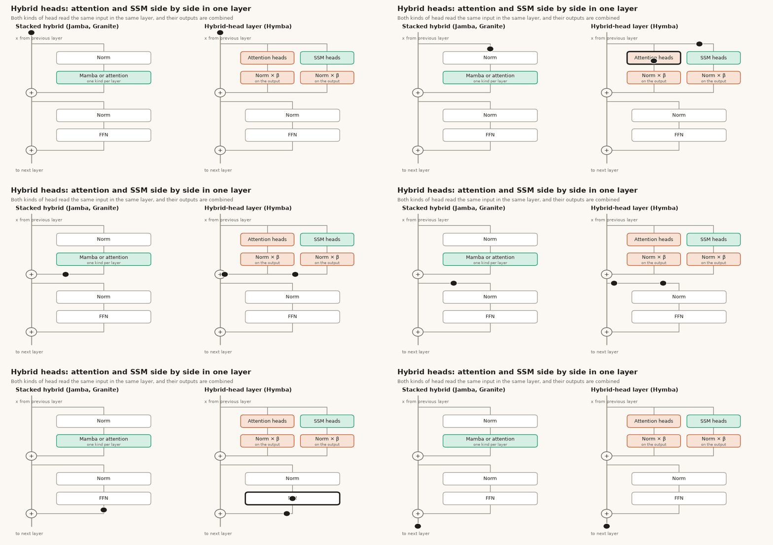
Hymba (Dong et al., 2024, NVIDIA) puts attention heads and state-space heads in the same layer, side by side, reading the same input. Each output is normalized and scaled before they are combined, because the SSM outputs were "consistently larger than those of the attention heads". At 300M parameters trained on 100B tokens, their Table 1 compares this parallel design with a sequential stack of the same parts: commonsense accuracy 45.19% vs 44.07%, recall 49.90% vs 45.16%. Hymba also uses sliding-window attention in most layers, keeping full attention in three.
The fifteen changes on one page
| # | Change | What it replaced | Reported benefit | Cost or limit |
|---|---|---|---|---|
| 1 | Post-LN block | (2017 original) | 28.4 BLEU En-De | needs warm-up (Xiong 2020) |
| 2 | Decoder only | encoder + decoder | one stack for text generation (our summary) | no source to cross-attend (our summary) |
| 3 | Pre-LN | Post-LN | no warm-up, 40% faster BERT pre-training | none stated; stream grows with depth (ours, measured) |
| 4 | RMSNorm | LayerNorm | 6.9% faster per step | none stated |
| 5 | Norm before and after | Pre-LN | "to stabilize training" | no number given |
| 6 | QK-norm | bias or soft-capping | stops logit blow-up at 8B (ViT-22B) | no number for LLMs |
| 7 | RoPE | learned position rows | 27.5 vs 27.3 BLEU | why it works not explained |
| 8 | NoPE | RoPE | better length generalization at 107M | not tested at scale |
| 9 | Parallel block | sequential block | about 15% faster training | small loss at 8B |
| 10 | SwiGLU | ReLU/GELU FFN | 1.636 vs 1.677 log-perplexity | none stated |
| 11 | MoE FFN | one FFN | up to 7x faster pre-training | memory holds all experts |
| 12 | Mamba | attention + FFN | 4-5x inference throughput | weaker in-context format following |
| 13 | Mamba-2 | Mamba scan | 2-8x faster scan | recall still limited by state |
| 14 | Hybrid stacks | all attention or all Mamba | 8.26 vs 8.60 perplexity at 350M | some layers keep a growing cache (ours, calculated) |
| 15 | Hybrid heads | stacked hybrid | 45.19 vs 44.07 commonsense at 300M | none stated; more parts per layer (our reading) |
Each benefit is the paper's own number, in its own setup, and so is each cost not marked "ours". What we ran is the code: all of it is in the repro bundle, and each block function reproduces its model's layer to rounding error.
Change one cell yourself
verify.py in the repro bundle below downloads the seven models from Hugging Face, records what goes into and comes out of each layer, and compares that with the block functions in blocks.py. It runs on a CPU. The easiest start is to change one line in a block function. In GPT-2's pre_ln_block, move the norm to after the addition and you have a Post-LN block; the gap from the real layer's output shows up at once. In the same way you can take RoPE out of qwen3_block.
If you want new posts in your inbox, the newsletter form is below.
Files for this post
Reproduction package
The harness, raw logs and result CSVs behind this post. No account needed; the README has a command that recomputes the tables without a GPU.
block-variants-repro.zip · 33 KB