28 Attention Designs, Each With a GIF and a Short Function: From Bahdanau to Latent Sparse Attention

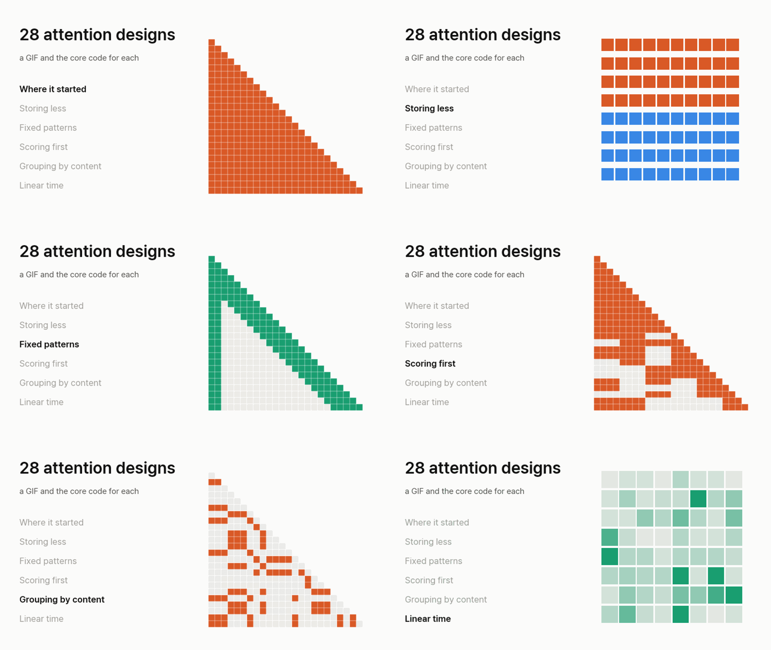
28 Attention Designs, Each With a GIF and a Short Function#

To pick the word after The capital of France is, a language model looks back at the earlier tokens and decides how much each one matters. That look-back is attention. It has been rebuilt many times since 2014, and the designs in this post each change one of four things: how a pair of tokens is scored, what stays in memory, which earlier tokens get read, or whether a list of earlier tokens exists at all.

This post walks through 28 designs in that order. Each one gets a GIF, a few sentences, three lines on what it improved, why and what it costs, and its core function in PyTorch, so you can see what changes from one design to the next.

Three words come up everywhere. The query is what the current token is looking for. A key is what an earlier token offers to be matched against. A value is what that token hands over when it matches. The KV cache is the list of stored keys and values, and its size is what many of these designs are trying to shrink.

Most GIFs share one grid. Rows are queries, columns are keys, and time runs downward, so a row shows which keys one token reads. Orange cells are read, green cells are always read, light blue cells are scored but not read, and grey cells are skipped. The inputs are random, so the picks illustrate the mechanism and measure nothing. Most GIFs are computed with the functions the post shows or the same formula. The alignment, storage, cross-attention, Linformer, ClusterKV and LSA GIFs are schematic.

What the code is. These are teaching versions for one request, without batching or speed tricks. We ran all of them on CPU with these kinds of checks: tensor shapes, whether a design reads the future when it should not, and limits where one design must equal a simpler one. We also read each named paper against its function and list what we left out. We did not train any of them and did not measure speed or accuracy. Numbers below are the papers' own unless we say otherwise.

How to read the numbers. Each number comes with its own paper's baseline, data and hardware, so compare it only with the baseline named beside it and not with numbers in other entries. Where a paper gives no number or names no cost, we say so. The "why" lines explain each design's mechanism in our own words, so they are not always the reason a paper states. Where we add an explanation of our own, we mark it as our reading.

What is in the list. Designs for text models that have a named paper or ship in a model we could check. We left out vision-only attention and tricks such as FlashAttention that compute the same result faster. So this is a selection and not every attention ever published.

Where it started: how a pair is scored#

1. Additive attention (Bahdanau, 2014)#

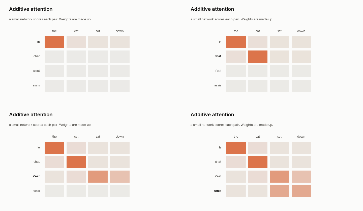
Translation models used to squeeze the whole source sentence into one vector. Bahdanau et al. let the decoder look back at every source word and learned that alignment jointly with the translation. A small network scores each pair. Here s is the decoder's previous state and h holds the states of a bidirectional encoder.

• What improved. Long sentences stopped falling apart. On English to French, the model reached BLEU 26.75 (a translation score, higher is better) against 17.82 for the fixed-vector model, both trained on sentences of up to 50 words, and it showed no drop on sentences of 50 words or more.
• Why it works. The decoder no longer has to fit a whole sentence into one vector, so the start of a long sentence stays reachable at every step.
• What it costs. A weight for every source word at every target word. The paper says this is not severe at 15 to 40 words but may limit other tasks, and it reports no timing.

def additive(s, h, W1, W2, v):
    """s: decoder state [d], h: encoder states [T, d]. Bahdanau: a small network scores each pair."""
    scores = v(torch.tanh(W1(s) + W2(h))).squeeze(-1)
    a = scores.softmax(-1)
    return a @ h, a

2. Multiplicative attention (Luong, 2015)#

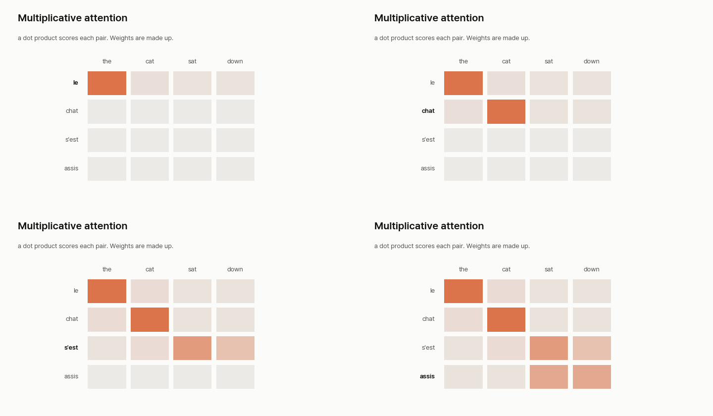
Luong et al. replaced the small network with a dot product, or a dot product with one learned matrix in between (their "general" form). It is simpler, and it scores with the decoder's current state, where Bahdanau used the previous one.

• What improved. Scoring got simpler without getting worse. On English to German, global dot scored BLEU 18.6 against 18.1 for the paper's location-based baseline (20.5 against 19.3 with unknown-word replacement). Its best local model reached 19.0 (20.9).
• Why it works. Our reading: a dot product needs no extra network for each pair and measures similarity directly. The paper itself gives no speed comparison.
• What it costs. No form wins everywhere. Global general scored 17.3 (19.1), and local-m with dot failed to train, with perplexity above 7.0. Perplexity measures how surprised a model is by the next word, so lower is better.

def luong(s, h, W=None):
    """Luong: score with a dot product, or with one matrix in between ("general"). s is the current state."""
    scores = h @ (s if W is None else W.T @ s)
    a = scores.softmax(-1)
    return a @ h, a

3. Scaled dot-product attention (Vaswani, 2017)#

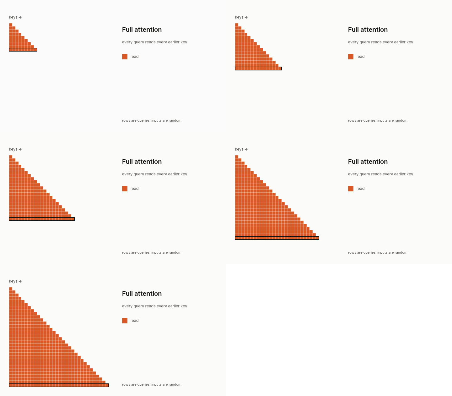
Attention Is All You Need made queries, keys and values three separate projections and divided scores by the square root of the dimension (Eq. 1). Almost everything below reuses this function. The optional read mask is how the sparse designs plug in: it tells each query which keys it may see. The triangle in the GIF is what is called full attention, and it is the baseline the rest are compared with.

• What improved. Dot-product scoring stayed usable at large dimensions, where the unscaled form fell behind additive attention. The paper gives no number for the scaling alone. Its 28.4 BLEU belongs to the whole model.
• Why it works. The paper suspects large dot products push softmax into regions with very small gradients, and the division counters that. The score stays plain matrix multiplication, which is fast in practice.
• What it costs. The paper names none for scaling. Every query still compares itself with every earlier key, so a layer's work grows with the square of the length.

def attend(q, k, v, read=None):
    """q [..., Q, d], k and v [..., T, d]. read is an optional boolean mask [Q, T]."""
    scores = q @ k.transpose(-1, -2) / math.sqrt(k.shape[-1])
    if read is not None:
        scores = scores.masked_fill(~read, float("-inf"))
    return scores.softmax(-1) @ v

4. Multi-head attention (Vaswani, 2017)#

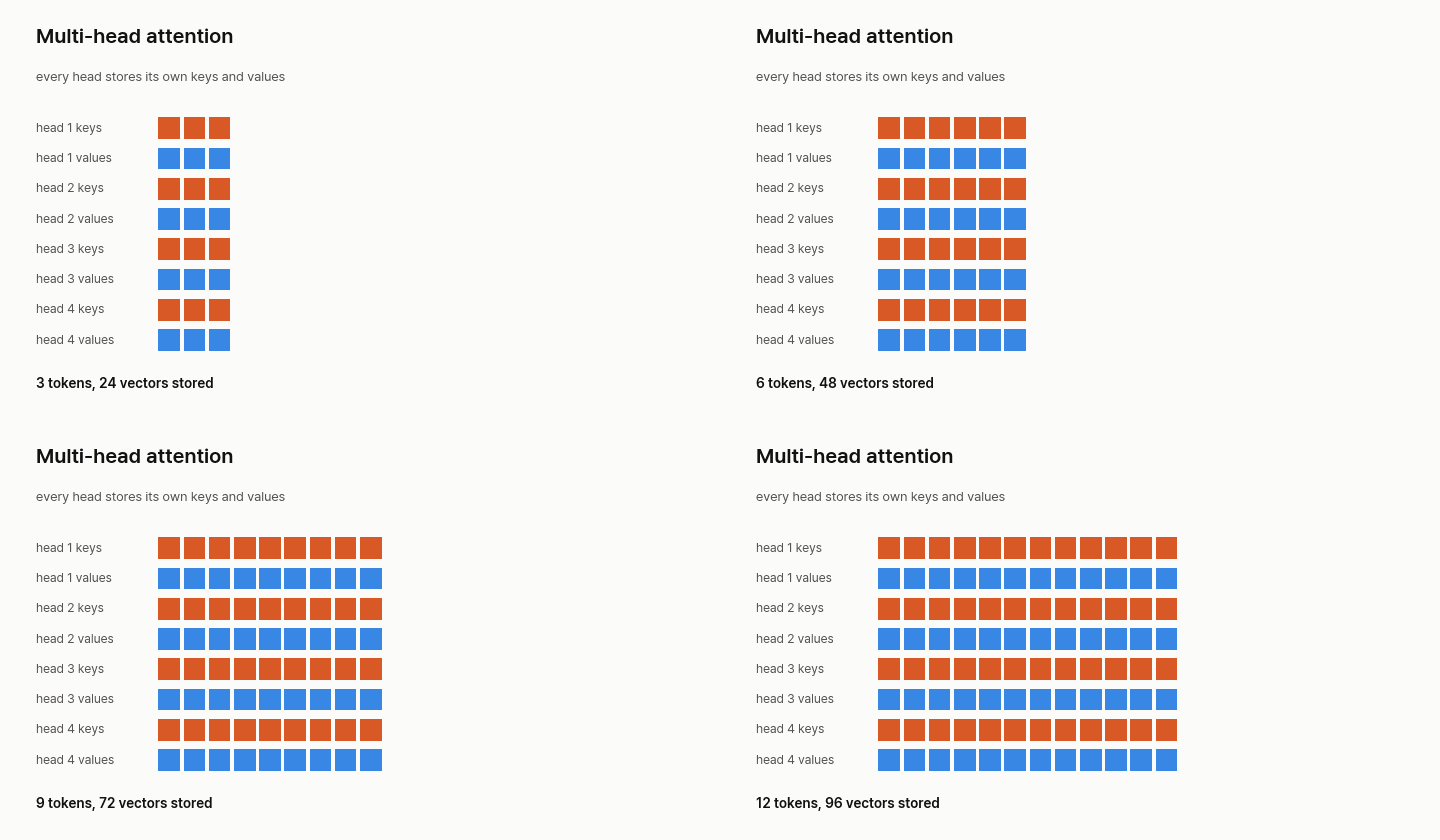
The same paper splits each vector into several heads that attend independently, then joins the results. Every head stores its own keys and values, which is why the KV cache grows so quickly. In our overview of current models, Llama 2 7B (32 query heads and 32 KV heads) and Gemma 7B (16 and 16) use this plain form.

• What improved. A model can attend to different kinds of information at the same time. The paper gives no separate number for this.
• Why it works. One head's averaging inhibits this, the paper says. Eight heads of 64 dimensions look through different projections, and each head is small enough that the total compute stays close to one full-size head.
• What it costs. A full set of keys and values is stored for every token. The paper names no memory cost, but DeepSeek-V2 later calls the KV cache a large bottleneck in deployment.

def mha(x, Wq, Wk, Wv, Wo, heads, read=None):
    """Every head keeps its own keys and values."""
    T, d = x.shape
    split = lambda t: t.view(T, heads, d // heads).transpose(0, 1)   # [heads, T, d/heads]
    out = attend(split(Wq(x)), split(Wk(x)), split(Wv(x)), read)
    return Wo(out.transpose(0, 1).reshape(T, d))

5. Cross-attention (Vaswani, 2017)#

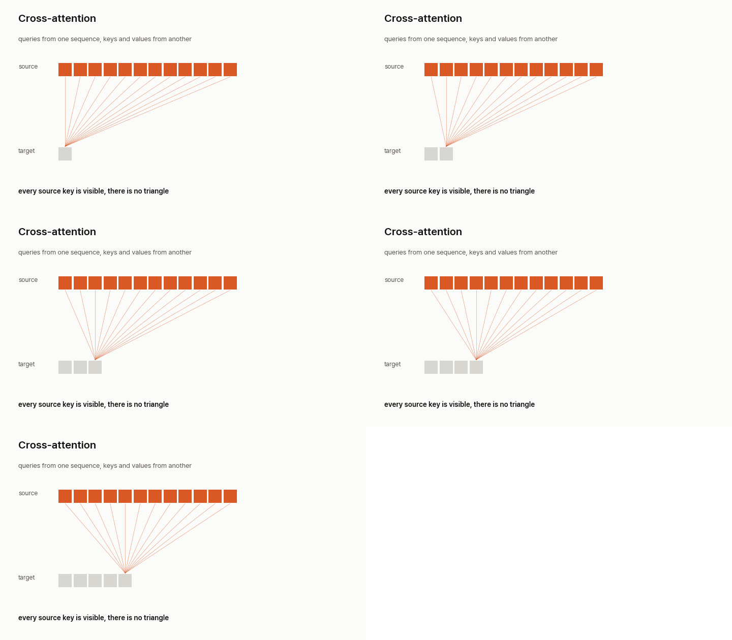
Queries come from one sequence and keys and values from another. The paper uses this between encoder and decoder, and there is no triangle, because every source token already exists. This is the same attend with different inputs.

• What improved. A decoder can use the attention idea from translation with no recurrent network underneath. The paper gives no separate number.
• Why it works. Queries come from the decoder and keys and values from the encoder, so the same function works across two sequences.
• What it costs. Our calculation: every decoder position reads every input position, so the work grows with the product of the two lengths, and the encoder output stays in memory while decoding.

def cross(x_dec, x_enc, Wq, Wk, Wv):
    """Queries from one sequence, keys and values from another. No triangle: every source token is visible."""
    return attend(Wq(x_dec), Wk(x_enc), Wv(x_enc))

Storing less: every key is still read#

These three change the memory bill and leave the reading pattern alone.

6. Multi-query attention (Shazeer, 2019)#

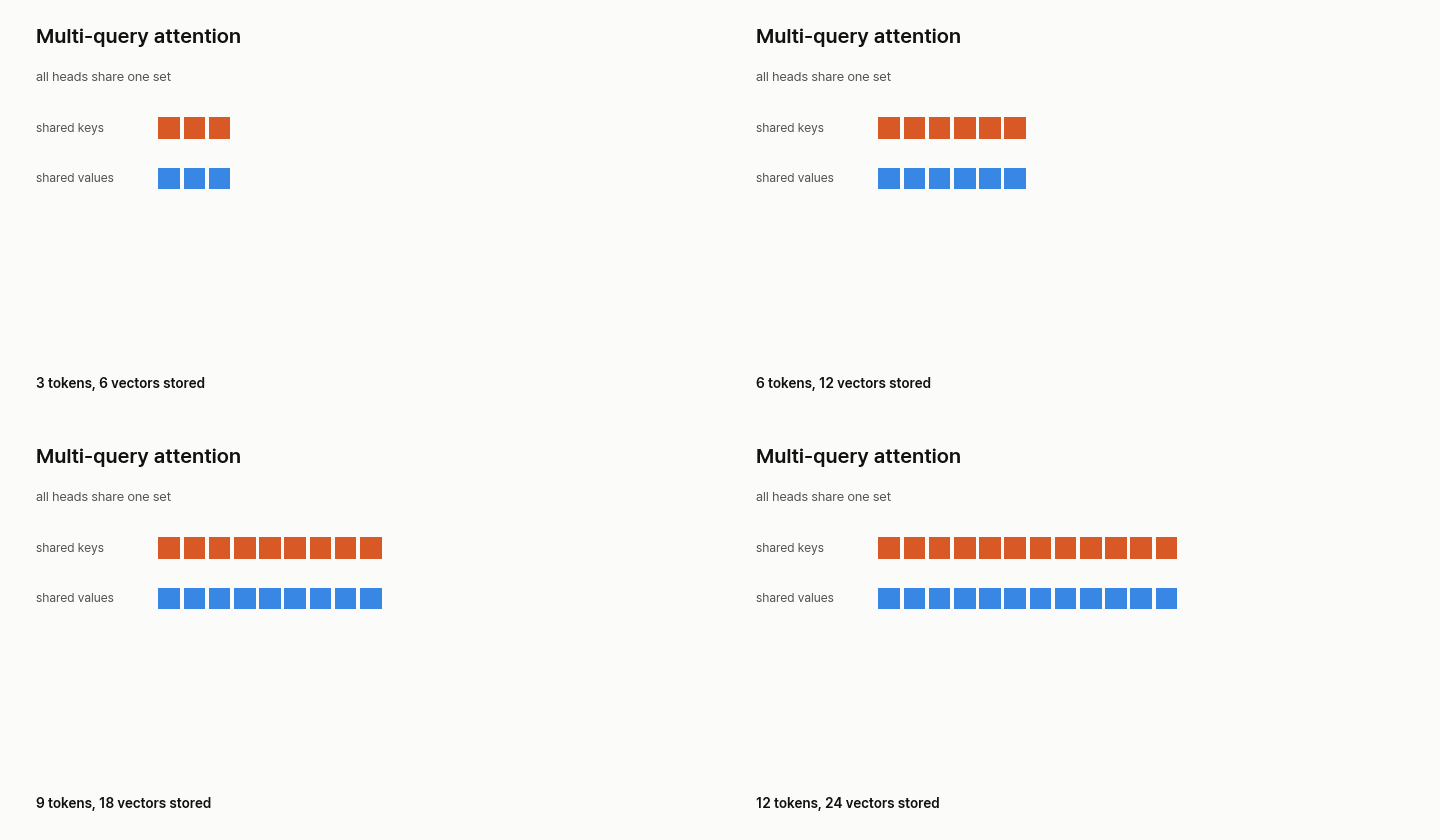
Shazeer kept many query heads and had them share a single set of keys and values, so only one key and one value per token is stored. Falcon 7B and Gemma 3 1B do this, according to the configs in our overview.

• What improved. Decoding got much faster. The decoder went from 46 to 3.8 µs per token, and beam search of width 4 from 203 to 32 µs (TPUv2 time, WMT14 English to German, length 128).
• Why it works. Reloading keys and values from memory at every step is the hard part of decoding, the paper argues, and sharing them shrinks that load by the number of heads.
• What it costs. Capacity. To keep parameter counts equal, the paper widened the feed-forward layer from 4096 to 5440, and BLEU stayed close (27.5 and 28.5 against 27.7 and 28.4, greedy and beam). Later results on bigger models are less kind: DeepSeek-V2's 7B dense comparison reports MMLU accuracy of 37.9 for MQA, 41.2 for GQA and 45.2 for MHA.

def mqa(x, Wq, Wk, Wv, Wo, heads):
    """Heads differ only in the query. One key and one value per token are stored."""
    T, d = x.shape
    q = Wq(x).view(T, heads, d // heads).transpose(0, 1)
    k, v = Wk(x)[None], Wv(x)[None]                                  # [1, T, d/heads], shared by broadcast
    return Wo(attend(q, k, v).transpose(0, 1).reshape(T, d))

7. Grouped-query attention (Ainslie, 2023)#

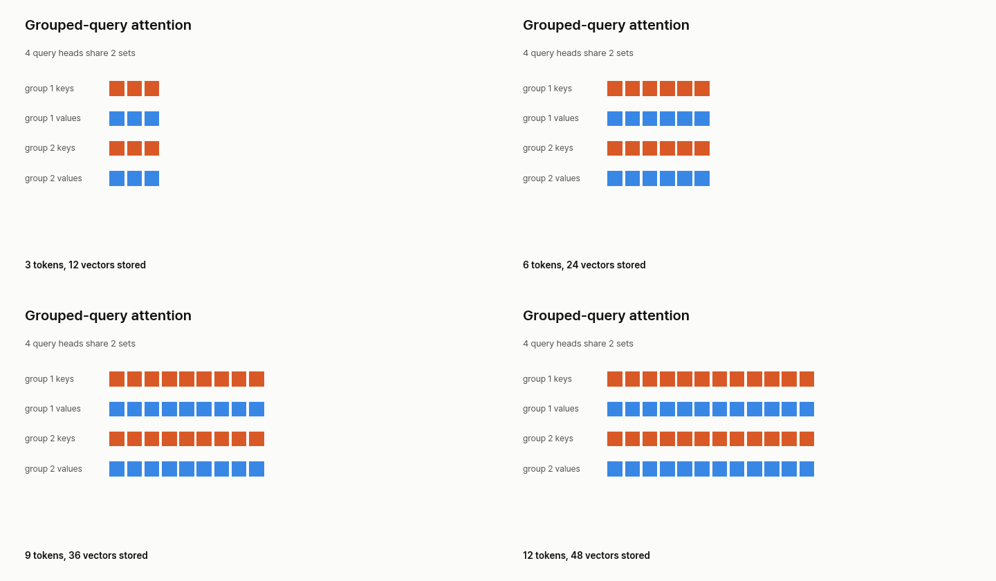
Ainslie et al. sit between the two: G groups, each sharing one key head and one value head. Our CPU check confirms both ends: groups=heads returns the same output as MHA, and groups=1 returns the same output as MQA when they share weights. Among the 2024 and later dense models in our overview (those that read every key), this is the most common form.

• What improved. Most of MQA's speed with nearly MHA's quality. On T5-XXL, GQA-8 takes 0.28 seconds per sample per TPUv4 chip and averages 47.1 across seven tasks (summarization, translation and QA). Original MHA takes 1.51 and averages 47.2, and MQA takes 0.24 and averages 46.6. GQA and MQA were converted from MHA and then trained for another 5% of the original steps.
• Why it works. The paper's explanation: in larger models the KV cache's memory bandwidth constrains speed less, and more heads make the cut in key-value size sharper. So going from one group to a few slows inference only modestly.
• What it costs. Each added group makes inference slower, gently at first and more steeply near MHA. DeepSeek-V2 also finds that GQA shrinks the cache but does not reach MHA's quality (41.2 against 45.2 in the previous entry, whole models).

def gqa(x, Wq, Wk, Wv, Wo, heads, groups):
    """In between: `groups` sets of keys and values, each shared by heads/groups query heads."""
    T, d, h_d = *x.shape, x.shape[1] // heads
    q = Wq(x).view(T, heads, h_d).transpose(0, 1)
    k = Wk(x).view(T, groups, h_d).transpose(0, 1).repeat_interleave(heads // groups, 0)
    v = Wv(x).view(T, groups, h_d).transpose(0, 1).repeat_interleave(heads // groups, 0)
    return Wo(attend(q, k, v).transpose(0, 1).reshape(T, d))

8. Multi-head latent attention (DeepSeek, 2024)#

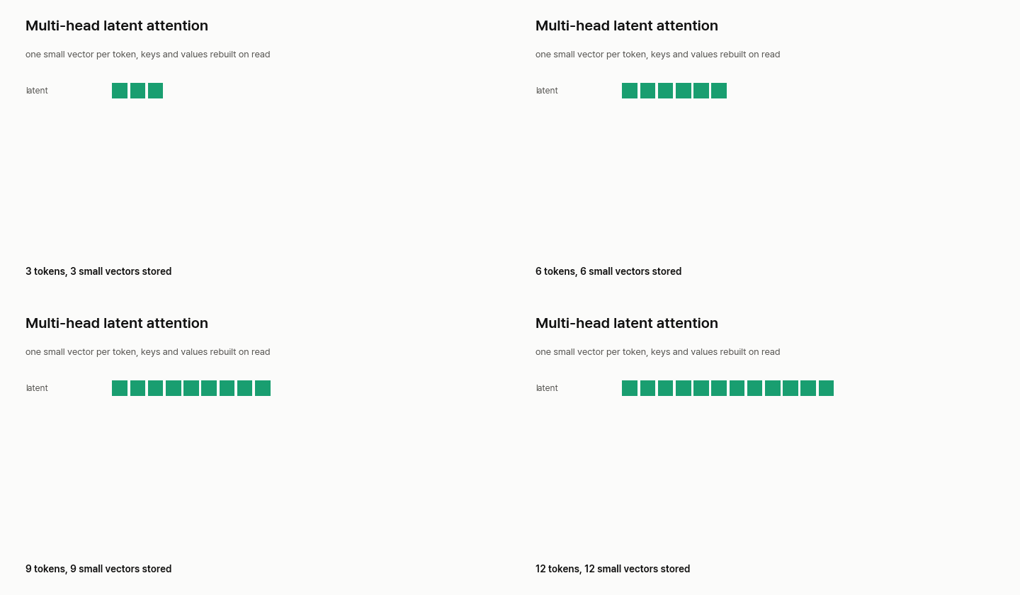
DeepSeek-V2 stores one small vector per token and rebuilds keys and values from it when reading. The paper reports a 93.3% smaller KV cache than DeepSeek 67B; that is a comparison between two whole models. Our function leaves out the query compression (Eqs. 12-13) and the small extra key that carries position information (RoPE, a rotary position encoding), which is cached too (Eq. 15), so real caches are larger than cache alone.

• What improved. KV cache per token. The Small MoE model went from 110.6K with MHA to 15.6K (14%) and the Large MoE from 860.2K to 34.6K (4%). These are similar-size whole models, and their parameter counts are not identical.
• Why it works. The paper compresses keys and values jointly into one low-rank vector and caches only that. Learned matrices map it back, so each head still reads its own keys and values.
• What it costs. RoPE does not fit the compressed form, so a separate position key has to be cached too, and the design adds an extra RMS Norm. Compressing the query does not shrink the cache at all.

def mla(x, Wq, Wc, Wuk, Wuv, Wo, heads):
    """Store one small vector per token. Keys and values are rebuilt from it when read. Leaves out the query
    compression and the small extra key that carries RoPE, which is also cached."""
    T, d = x.shape
    cache = Wc(x)                                                    # [T, small]: all that is kept, without RoPE
    split = lambda t: t.view(T, heads, d // heads).transpose(0, 1)
    out = attend(split(Wq(x)), split(Wuk(cache)), split(Wuv(cache)))
    return Wo(out.transpose(0, 1).reshape(T, d))

Fixed patterns: the mask is decided in advance#

From here on, keys get skipped. In the next six designs, position alone decides which ones. causal(n) below is a lower-triangular mask: a token sees itself and everything before it.

9. Sliding window#

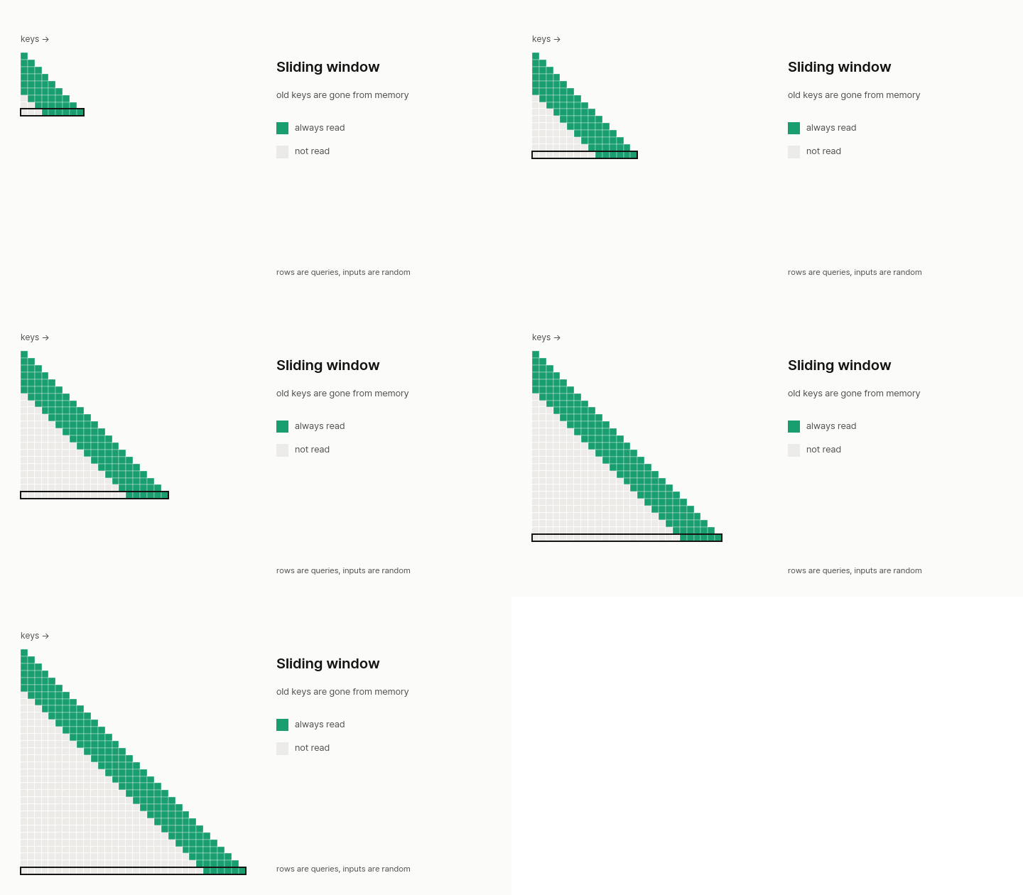
Each query reads its latest window keys, and older keys can leave memory. The cache stops growing, and anything older than the window is gone. It has no single source paper.

• What improved. Memory stops growing, and a token's work stops depending on context length. In the MQA paper, one model reading the current and previous 31 positions went from 46 to 23 µs per token, and from 203 to 47 µs in beam search, with BLEU 27.5 and 28.3 against 27.7 and 28.4. That is the nearest number we have, since there is no single source paper.
• Why it works. Our reading, since there is no source paper: each query reads a fixed number of keys, however long the context gets.
• What it costs. What leaves the window is gone, and this can break a model outright. The sinks paper reports perplexity 5158.07 on PG-19 for Llama-2-13B with a window of 1024 and the first tokens evicted. In the LSA paper's 128K training comparison on one small hybrid model, a window of 2,560 keys plus 4 sink keys scores 3.0 on RULER (a long-context test, higher is better), against 34.7 for full attention.

def sliding(n, window):
    """Each query reads its latest `window` keys. Older keys can be dropped from memory."""
    i, j = torch.meshgrid(torch.arange(n), torch.arange(n), indexing="ij")
    return (j <= i) & (j > i - window)

10. Attention sinks (Xiao, 2023)#

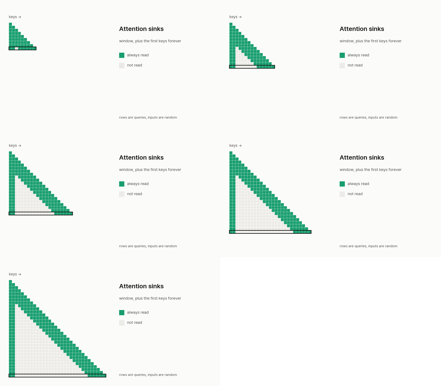
Xiao et al. found that models keep placing attention on the very first tokens, so evicting those hurts far more than their content would suggest. Their fix keeps a few of them forever, and the paper says just 4 initial tokens suffice. Latent Sparse Attention (LSA, entry 22) carries the same always-read strip.

• What improved. Long streaming generation stopped breaking. On the same test, keeping 4 first tokens plus a window of 1020 took perplexity from 5158.07 to 5.40, and it runs up to 22.2x faster per token than a sliding window that recomputes the cache.
• Why it works. Softmax weights must add up to one, the paper explains, so attention with nowhere useful to go gathers on the first tokens. Keeping them keeps that distribution stable.
• What it costs. The paper says it directly: this does not extend the context or add long-term memory. Older tokens are still gone.

def sink(n, window, sinks=4):
    """Sliding window, but the first few keys stay forever. Attention keeps landing on them."""
    read = sliding(n, window)
    read[:, :sinks] = True
    return read & causal(n)

11. Local-global layers#

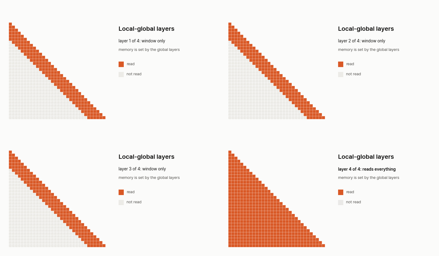
Most layers read a window and every few layers one reads everything, so at long context memory is set mostly by the full layers. There is no single paper for this either, and the mix varies a lot: our overview lists Gemma 2 at one in two, Gemma 3 at one in six and gpt-oss at one in two with a window of 128.

• What improved. Most layers get cheap while far tokens stay reachable. There is no source paper for this mix. The nearest numbers we found are from a different mix, local attention with content-routed heads in Routing Transformer: on CIFAR-10 with a window of 512, local only gives 3.009 bits/dim at 9.023 steps/s, 4 routing heads in 2 layers give 2.986 at 7.409, and full attention gives 2.983 at 5.608. Lower bits/dim is better.
• Why it works. Our reading: window layers handle nearby context cheaply, and the occasional full layers carry far information across the model.
• What it costs. The ratio is a real trade-off. In Kimi Linear, a mix of linear and full layers, 7 to 1 gave worse validation and 1 to 1 gave more inference overhead. The LSA paper adds a limit from the other side: making the global layers faster helps only those layers.

def layer_read(layer, n, window, global_every):
    """Most layers read a window, every few layers one reads everything."""
    return causal(n) if (layer + 1) % global_every == 0 else sliding(n, window)

12. Sparse Transformer (Child, 2019)#

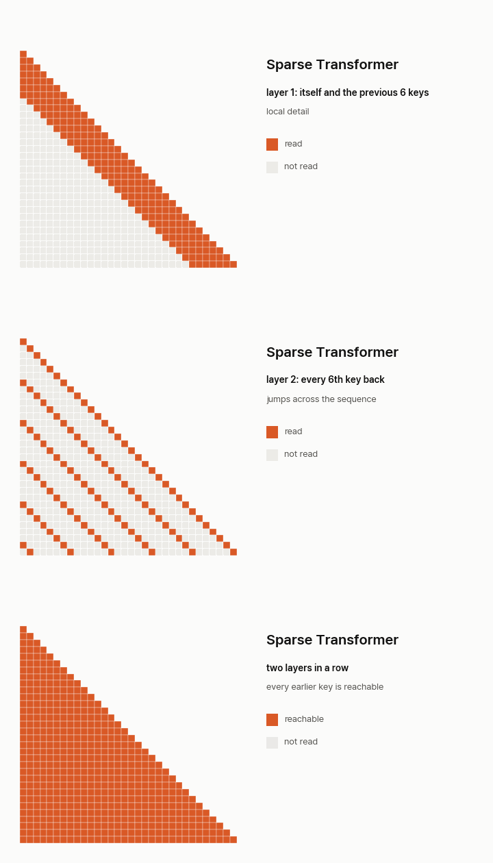
Child et al. alternate two masks: one layer reads the recent keys and the next reads every stride-th key, at O(n√n) cost. Our check confirms the two masks together can reach every earlier key in two hops. The paper also says this strided pattern "can fail to properly route information" on text.

• What improved. Long sequences at dense-model quality for less computation. On CIFAR-10, strided attention scored 2.80 bits/dim against 2.82 for dense (lower is better). On Enwik8, a fixed pattern with 95M parameters reached 0.99, against 1.03 for Transformer-XL at 88M and 0.99 at 277M.
• Why it works. Two hops reach every earlier key, so each layer can read only about √n keys and still connect everything.
• What it costs. The fixed pattern used on text costs c times the strided one, with c of 8, 16 or 32 in the paper, which gives back part of the saving. Routing Transformer later points out that fixed patterns limit which tokens can be pooled, because content plays no part.

def sparse_transformer(layer, n, stride):
    """Strided pattern. One layer reads itself and the previous `stride` keys, the next reads every stride-th key back.
    Together the two layers can reach any earlier key."""
    i, j = torch.meshgrid(torch.arange(n), torch.arange(n), indexing="ij")
    same = (j >= i - stride) if layer % 2 else ((i - j) % stride == 0)
    return same & causal(n)

13. Longformer (Beltagy, 2020)#

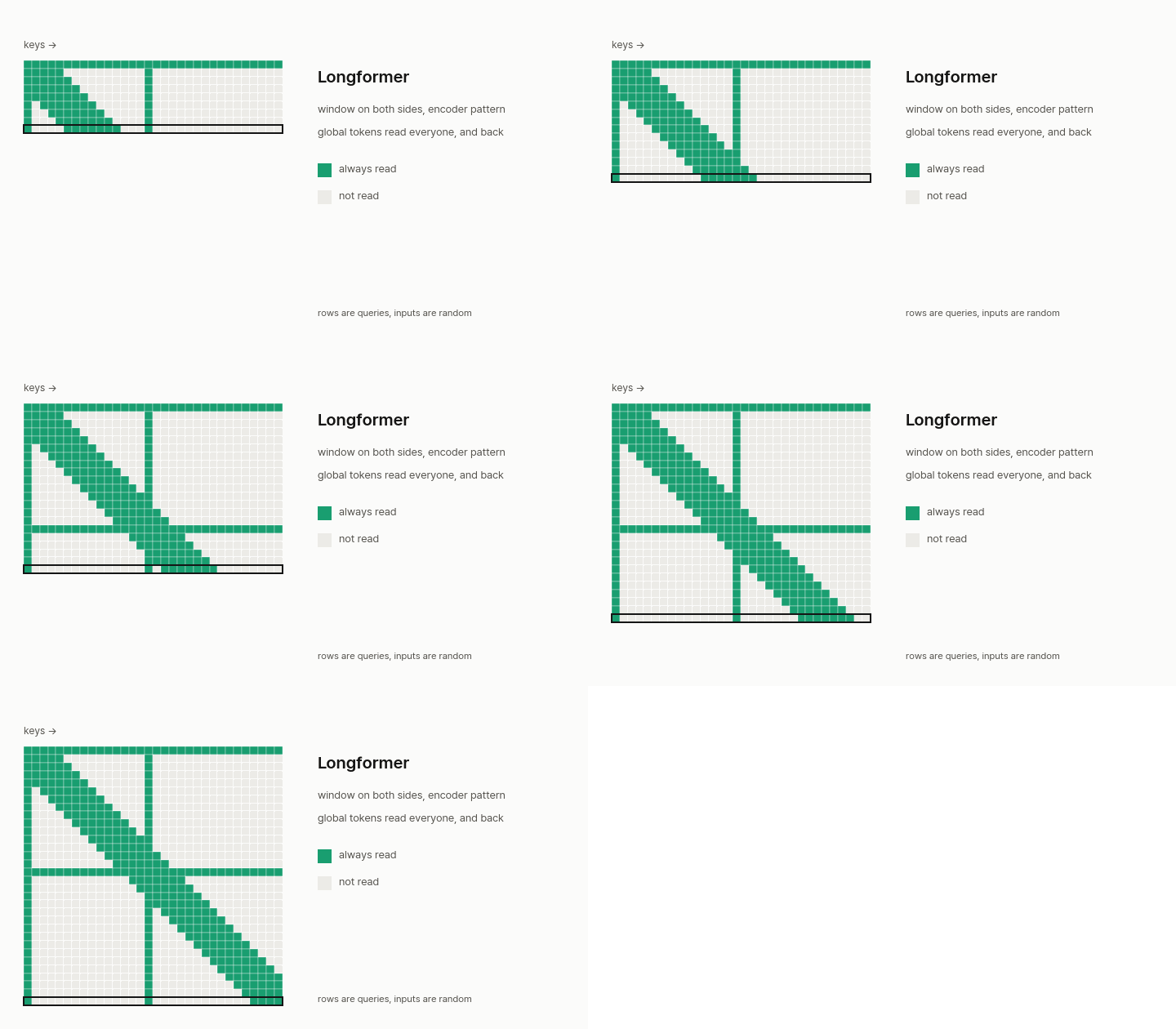
Longformer combines a window of half window on each side with a few global tokens that read everyone and are read by everyone. This is an encoder pattern, so the grid is square and tokens see the future. For causal language modeling the paper describes dilated windows, which skip keys at even gaps, on 2 heads of the higher layers, and does not mention global tokens. Its encoder-decoder version keeps full self-attention in the decoder. We omit the separate projections it uses for global attention.

• What improved. Long documents can be read whole. On dev sets, WikiHop accuracy was 73.8 against 72.4 for RoBERTa-base (75.0 with 15 epochs), and Hyperpartisan F1 was 94.8 against 87.4.
• Why it works. The window handles local context, and global tokens carry what the whole document needs. The paper tested removing them: without global attention and its linear projection, WikiHop fell to 65.5, 8.3 points below 73.8 at length 4,096.
• What it costs. Language modeling needs a schedule that learns local context first, and the encoder-decoder version keeps full self-attention in the decoder, so that side stays quadratic.

def longformer(n, window, global_ids):
    """A window on both sides, plus a few global tokens that read and are read by everyone. Encoder pattern."""
    i, j = torch.meshgrid(torch.arange(n), torch.arange(n), indexing="ij")
    read = (i - j).abs() <= window // 2
    read[:, global_ids] = True
    read[global_ids, :] = True
    return read

14. BigBird (Zaheer, 2020)#

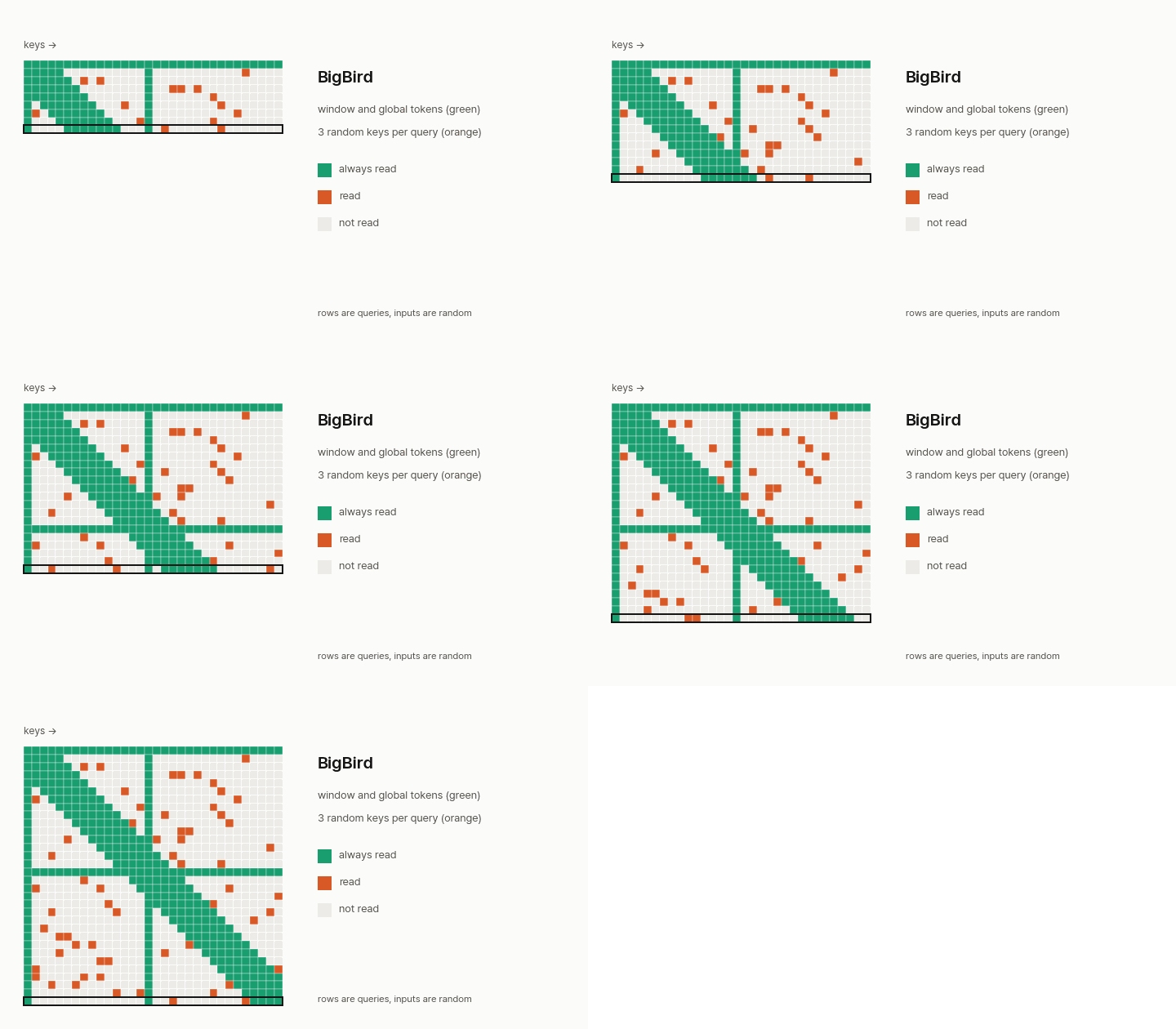
BigBird adds random keys to the window and the global tokens. The random links come from graph theory, where they keep paths between tokens short. The proofs lean on the global tokens: the paper shows that any sparse pattern containing a star graph through a global token is a universal approximator of sequence functions, meaning it can approximate them as closely as needed, and that a sparse encoder and decoder can simulate any Turing machine. In its experiments the decoder uses full self-attention, and the real implementation works on blocks of tokens, where our function picks single keys.

• What improved. Sequences up to 8x longer than before. Among its test results against Longformer, TriviaQA Verified is 92.4 against 85.3, while HotpotQA ties at 81.2 and WikiHop is close at 82.3 against 81.9. So the gain varies by task. On Arxiv classification it is about 5 points above the state of the art of the time.
• Why it works. Random links keep paths between tokens short, so information can cross the sequence in few layers, and the global tokens are what the proofs rest on.
• What it costs. The paper states a "no free lunch" result: there is a task where sparse attention needs polynomially more layers than full attention. Its decoder also stays on full self-attention.

def bigbird(n, window, global_ids, r, seed=0):
    """Longformer's two parts, plus r random keys per query. Encoder pattern; the real code works on blocks."""
    g = torch.Generator().manual_seed(seed)
    read = longformer(n, window, global_ids)
    for i in range(n):
        read[i, torch.randint(0, n, (r,), generator=g)] = True
    return read

Scoring first: a cheap indexer chooses#

Position no longer decides. Each query scores earlier tokens with something cheap, then reads the winners. Every key stays in memory, so these save compute and do not shrink the cache (DSA's indexer even adds a small key per token). That scoring step is also where the cost moves to, as our post on LSA shows.

15. DeepSeek Sparse Attention (2025)#

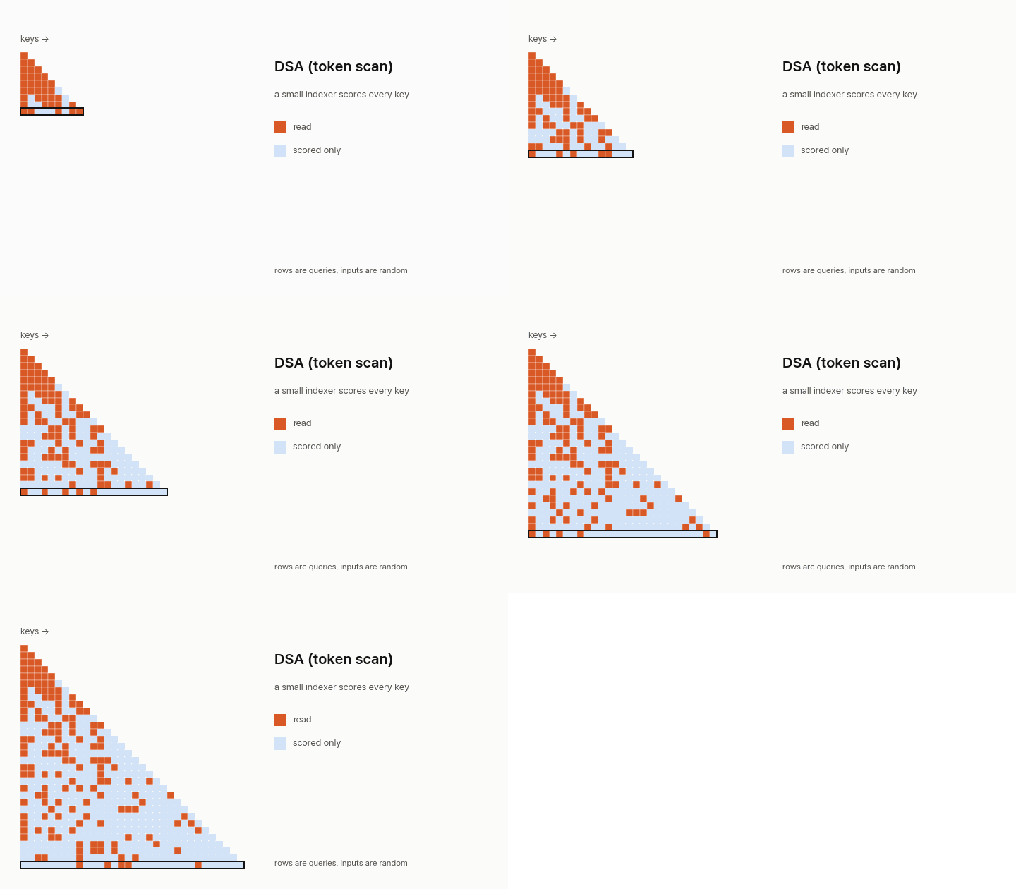
DeepSeek-V3.2 adds a small indexer with its own small query heads and one small key per token. ReLU keeps only positive matches, and attention reads the top 2,048. Every key is scored for every query, which the LSA paper calls token sparse attention. We call it a token scan. The GIF uses 5 keys so the picks are visible.

• What improved. Main attention goes from quadratic in length to L·k, where k is how many keys it reads. The one score we can quote is for the whole model: V3.2-Exp is 4 points above V3.1-Terminus on AA-LCR in reasoning mode. The paper gives no number for this attention alone.
• Why it works. A small indexer picks the top keys, so the expensive multi-head read runs only on those.
• What it costs. The indexer itself is still quadratic, though the paper says it is much cheaper than MLA. Training adds a stage where the indexer learns from a KL loss on frozen parameters.

def dsa_scores(qi, ki, w):
    """A small indexer scores every key. qi [H, Q, d]: small query heads, w [H, Q]: their weights, ki [T, d]."""
    return (w[:, :, None] * F.relu(qi @ ki.T)).sum(0)                # [Q, T], then keep the top k

16. MoBA (Lu, 2025)#

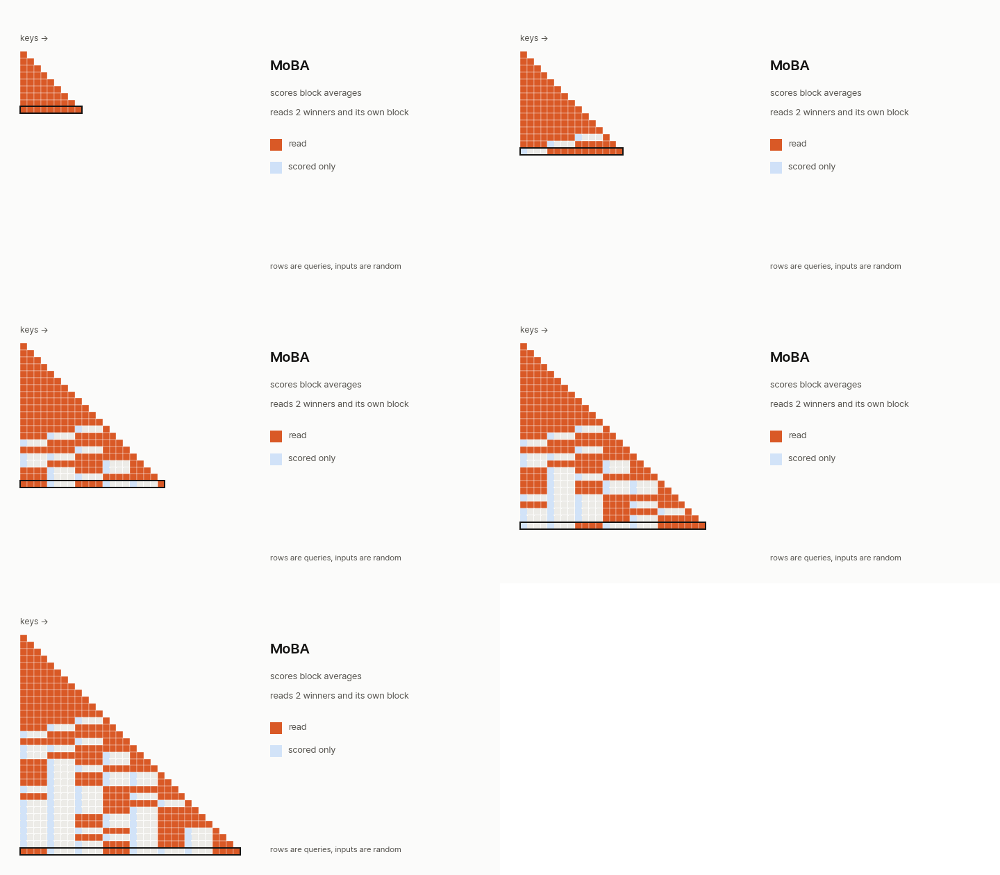
MoBA splits keys into blocks and scores each block's average, so it needs one score per block. With 64 blocks and the top 3, the paper reaches 95.31% sparsity, which is just 1 minus 3/64. The query's own block counts as one of those three. The paper selects per head, and we show one head.

• What improved. Up to 6.5x faster prefill at 1M than full attention, and 16x less attention computation at 10M. RULER at 128K stays at 0.7818 against 0.7849, with 62.5% sparsity.
• Why it works. Keys are averaged into blocks, so a query needs one score per block and reads only the winners.
• What it costs. Training with MoBA alone raises loss on the last tokens of a long sequence, and the paper's fix brings full attention back into the recipe. Each query also still scores every block, which is the cost the LSA paper goes after.

def moba_read(q, k, block, top):
    """Average each block of adjacent keys and score the averages. `top` counts the query's own block,
    which is always read. One head here; the paper selects per head."""
    Q, T = len(q), len(k)
    means = k.unfold(0, block, block).mean(-1)
    scores = q @ means.T
    read = torch.zeros(Q, T, dtype=torch.bool)
    for i in range(Q):
        closed = i // block                                          # blocks that lie fully in the past
        for b in scores[i, :closed].topk(min(top - 1, closed)).indices.tolist():
            read[i, b * block:(b + 1) * block] = True
        read[i, closed * block:i + 1] = True
    return read

17. Native Sparse Attention (Yuan, 2025)#

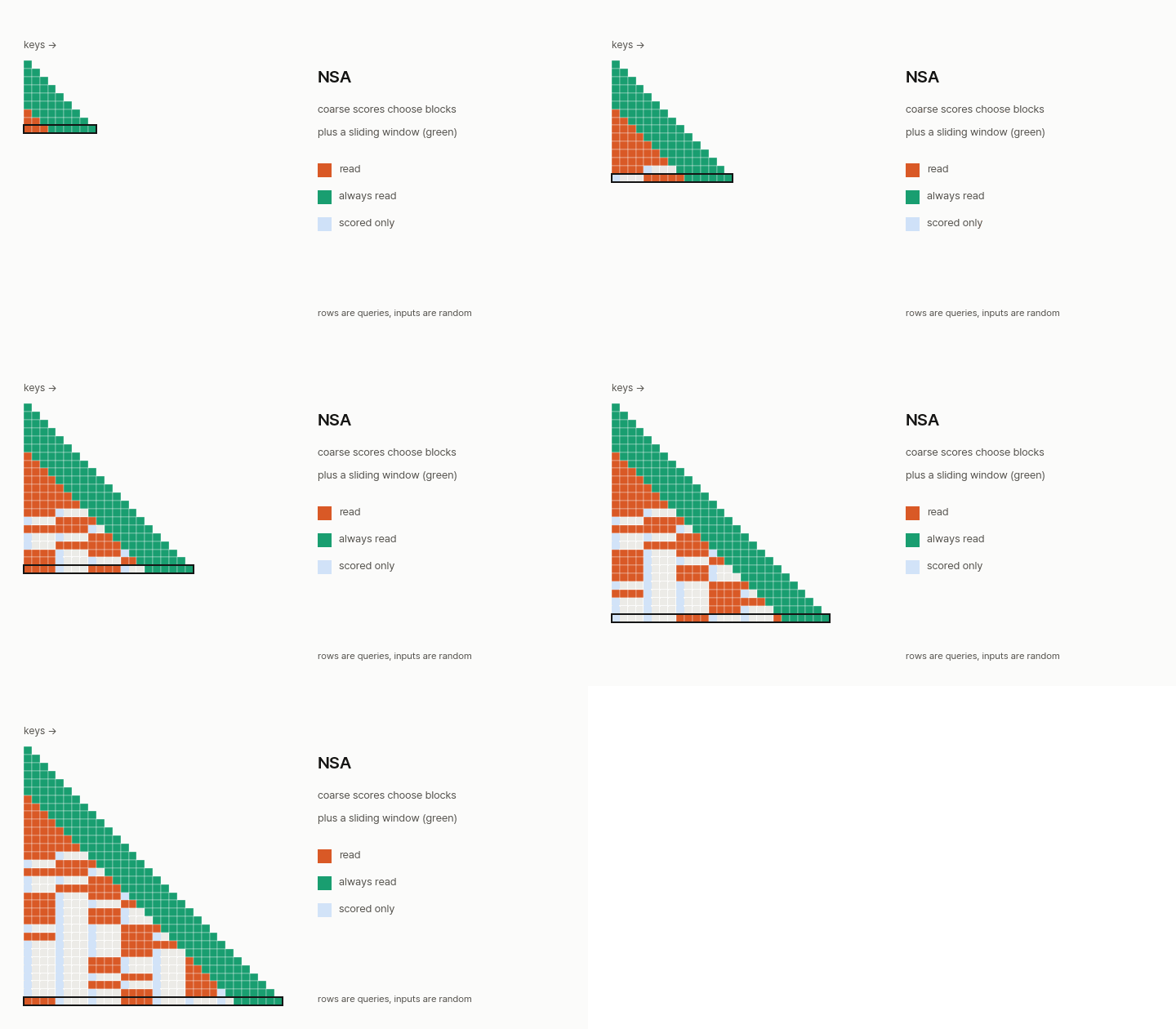
NSA mixes three gated branches: compressed blocks for an overview, selected blocks for detail, and a sliding window, and the whole selection is trained end to end with the model. The paper tests this on a 27B model. Our function shows only which keys get read. It uses a mean where the paper uses a small learned network, and it omits the gates and the separate keys and values per branch. The paper's compressed blocks overlap (length 32, stride 16); ours do not. When the paper picks its 16 blocks it always includes the first block and the 2 nearest ones; our function does not force the first block, and the sliding window covers the nearby keys.

• What improved. Far less memory is read. At 64K, one step accesses 5,632 tokens against 65,536, which the paper computes as an expected 11.6x (4x at 8K). That is calculated from access volume and not measured. LongBench averages 0.469 against 0.437 for full attention.
• Why it works. Three learned branches cover overview, detail and nearby context, and training the selection end to end lets it fit the model.
• What it costs. The LSA paper's later 128K training comparison puts NSA's validation loss at 1.117 against 1.085 for full attention, and RULER at 19.2 against 34.7, in that paper's setup. Every block is also still scored.

def nsa_read(q, kc, block, top, window):
    """Scores on pooled keys choose blocks, then fine attention reads those keys and a window. Mean pooling
    stands in for the paper's small learned network. The real model mixes a compressed branch, this selected
    branch and the window branch with learned gates, each with its own keys and values."""
    Q, T = len(q), len(kc)
    scores = q @ kc.unfold(0, block, block).mean(-1).T
    read = sliding(max(Q, T), window)[:Q, :T].clone()
    for i in range(Q):
        closed = i // block
        for b in scores[i, :closed].topk(min(top, closed)).indices.tolist():
            read[i, b * block:(b + 1) * block] = True
    return read

18. Block scan: CSA, QSA, GLM-5.3-Flash SA#

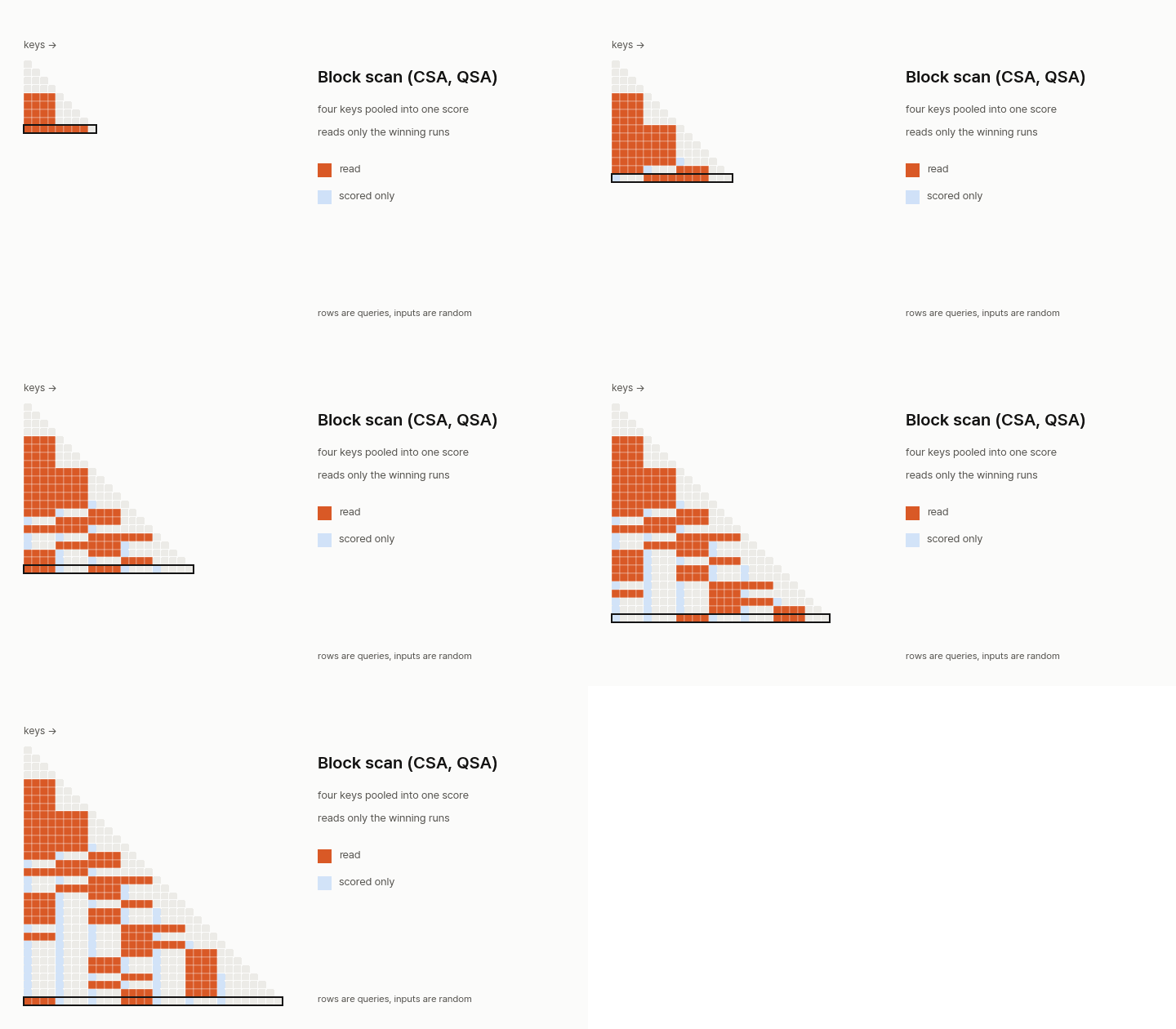
CSA, QSA and GLM-5.3-Flash SA are sparse layers from recent reports. They compress every four keys into one score, so a query does T/4 scores and reads whole runs. The LSA paper calls this block sparse attention. We have not read these reports directly: this sketch follows the description in the LSA paper, so treat it as the shape of the idea and not as any one model's code. That paper's parameter table lists no first keys or window for its flat block baseline, so our function has neither, and a query with no finished block reads nothing here.

• What improved. One query does T/4 scores where a token scan does T. That is the arithmetic of the design, and we found no standalone number for it.
• Why it works. As the LSA paper describes these layers, four keys compress into one score, and the winning run is read whole.
• What it costs. The scoring still grows with length. The LSA paper reports that at 10M tokens the indexer takes 98% of prefill in one GLM-5.3-Flash global attention layer, and it calculates that a free indexer would make that layer 58x faster in prefill and 8.9x in decode on one H200.

def block_scan_read(q, k, block, top):
    """One score per run of adjacent keys, taken from small index vectors. Read only the winning runs."""
    Q, T = len(q), len(k)
    scores = q @ k.unfold(0, block, block).sum(-1).T                 # pool: four keys summed into one
    read = torch.zeros(Q, T, dtype=torch.bool)
    for i in range(Q):
        closed = i // block
        for b in scores[i, :closed].topk(min(top, closed)).indices.tolist():
            read[i, b * block:(b + 1) * block] = True
    return read

SOTAAZ course

This course alone $79 · 24 lectures · first 3 freeWatch free →

Grouping by content: similar keys together#

A block holds whatever happened to sit nearby. These four group keys by what they contain, so a query can jump to related tokens anywhere.

19. Reformer (Kitaev, 2020)#

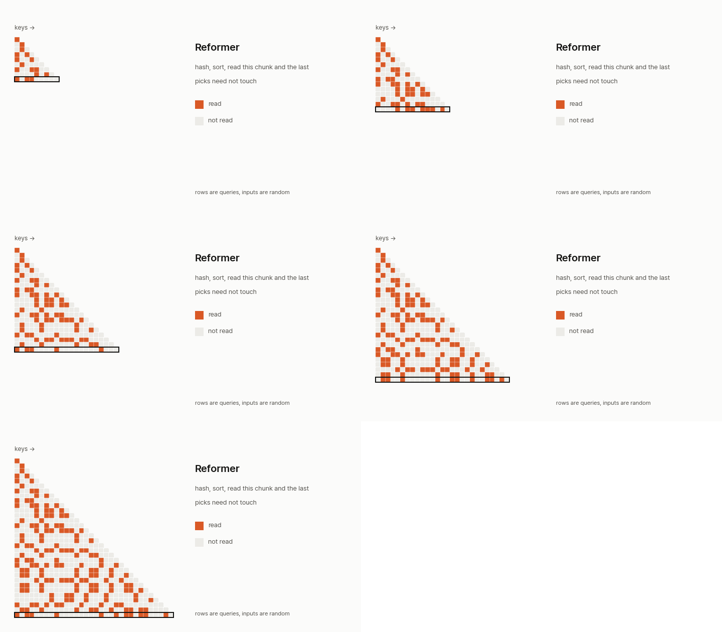
Reformer hashes with random rotations, h(x) = argmax([xR; -xR]), sorts positions by bucket and attends within a chunk of that order and the chunk before it. Queries and keys share one vector, and a token reads itself only when it has nothing else to read. The paper repeats the hashing over several rounds to miss fewer matches, and we show one round and omit key normalisation.

• What improved. Training on long sequences fits in memory. The paper notes that 64K tokens can exhaust an accelerator with ordinary attention. With total tokens held fixed, its hashed attention's speed stays flat as length grows, where regular attention slows, and a 12-layer model reached 1.05 bits/dim on enwik8.
• Why it works. Similar vectors tend to land in the same bucket, so a token reads only its chunk. Reversible layers save the rest of the memory by recomputing activations during training.
• What it costs. Accuracy depends on hashing rounds, with 8 almost matching full attention, and compute grows with each round. Routing Transformer later reports about 3.65 bits/dim for Reformer on ImageNet-64 against its own 3.43, and Linformer says the efficiency gains appear only above length 2,048.

def lsh_buckets(x, n_buckets, seed=0):
    """Random rotations: similar vectors tend to land in the same bucket. Queries and keys share one vector."""
    R = torch.randn(x.shape[-1], n_buckets // 2, generator=torch.Generator().manual_seed(seed))
    rotated = x @ R
    return torch.cat([rotated, -rotated], -1).argmax(-1)

def reformer_read(x, n_buckets, chunk, seed=0):
    """Sort positions by bucket, cut into chunks, attend within a chunk and the one before it. No token reads
    itself unless it has nothing else. One hash round here; the paper repeats it and combines the rounds."""
    order = torch.argsort(lsh_buckets(x, n_buckets, seed), stable=True)
    n = len(x)
    chunk_of = torch.empty(n, dtype=torch.long)
    chunk_of[order] = torch.arange(n) // chunk
    i, j = torch.meshgrid(torch.arange(n), torch.arange(n), indexing="ij")
    read = (chunk_of[j] == chunk_of[i]) | (chunk_of[j] == chunk_of[i] - 1)
    read = read & causal(n) & ~torch.eye(n, dtype=torch.bool)
    alone = ~read.any(1)
    read[alone, alone] = True
    return read

20. Routing Transformer (Roy, 2020)#

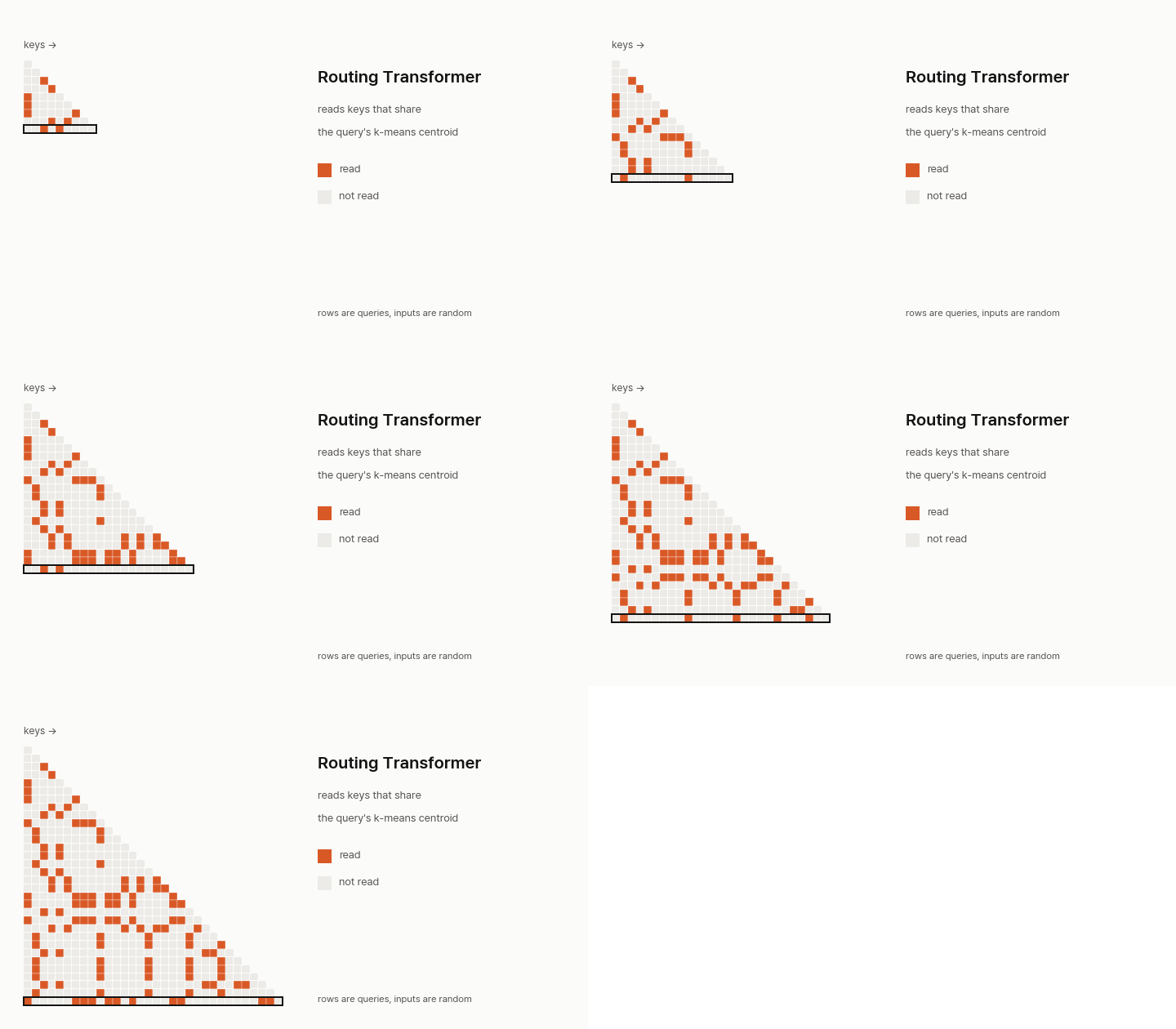
Roy et al. learn the groups as they go. Queries and keys join their nearest k-means centroid, and centroids follow the data by a moving average, at O(n^1.5 d) with √n centroids. The paper assigns with a balanced top-w, shares queries and keys under a causal mask and combines this with local attention; our function uses a plain argmax and separate q and k.

• What improved. Reading follows content where fixed patterns could only follow position. Perplexity on Wikitext-103 is 15.8 against 18.3 for Transformer-XL, and ImageNet-64 is 3.43 against 3.44 bits/dim for Sparse Transformer (lower is better for both).
• Why it works. Centroids that follow the data send a query to the keys most like it, wherever they sit.
• What it costs. Too much routing hurts. On CIFAR-10 at window 512, 8 routing heads in 12 layers gave 3.400 bits/dim at 3.062 steps/s, worse and slower than local only at 3.009 and 9.023. A good mix, 4 heads in 4 layers, gave 2.975 at 6.492.

def routing_read(q, k, centroids):
    """q and k are LayerNorm-ed. Each joins its nearest k-means centroid, and a query reads keys that share it.
    The paper assigns with a balanced top-w; argmax here is simpler."""
    cq, ck = (q @ centroids.T).argmax(-1), (k @ centroids.T).argmax(-1)
    return (cq[:, None] == ck[None]) & causal(max(len(q), len(k)))[:len(q), :len(k)]

def routing_update(centroids, q, k, decay=0.999):
    """Centroids follow the data by a moving average of the queries and keys assigned to them."""
    cq, ck = (q @ centroids.T).argmax(-1), (k @ centroids.T).argmax(-1)
    centroids = decay * centroids
    centroids.index_add_(0, cq, (1 - decay) / 2 * q)
    centroids.index_add_(0, ck, (1 - decay) / 2 * k)
    return centroids

21. ClusterKV (Liu, 2024)#

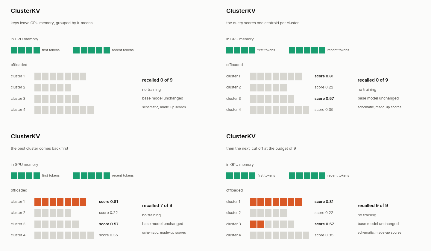
ClusterKV needs no training and leaves the model alone. It works purely as a cache at inference: keys leave GPU memory grouped by k-means, and each step recalls the best clusters until a budget is full. The paper reports negligible accuracy loss at a 32K context with a budget of 1K to 2K. It clusters each new batch of 320 generated tokens on its own, always keeps the first 16 tokens and starts with L/80 centroids, and we omit that bookkeeping.

• What improved. KV stays out of GPU memory with no retraining. LongBench's 8-dataset average at a budget of 1024 is 48.34, against 43.23 for Quest and 45.13 for InfiniGen, two earlier cache methods. Latency drops by up to half (up to 2x speedup) at a prompt of 32K, 1,024 decoded tokens and a budget of 1,024, and decode throughput rises by up to 2.5x.
• Why it works. Recall follows content, so the keys a query wants can come back wherever they sit in the context.
• What it costs. It stays below keeping everything at every budget: 46.69 at 256 and 48.7 at 2,048, against 49.01 for the full cache. Against InfiniGen on OPT-6.7B at a budget of 256, selection takes about 5% of decode latency. Clustering adds work too, at 6% to 8% of prefill and under 2% of total inference time.

def clusterkv_recall(q, kept, evicted, labels, centroids, budget):
    """An inference-time cache: keys leave GPU memory grouped by k-means, except the first tokens and recent
    ones. Each step scores the centroids and recalls keys from the best clusters until the budget is full.
    No training, and the base model is unchanged."""
    back = []
    for c in (q @ centroids.T).argsort(descending=True).tolist():
        back += (labels == c).nonzero().squeeze(-1).tolist()
        if len(back) >= budget:
            break
    return torch.cat([kept, evicted[back[:budget]]])

22. Latent Sparse Attention (Kubicek, 2026)#

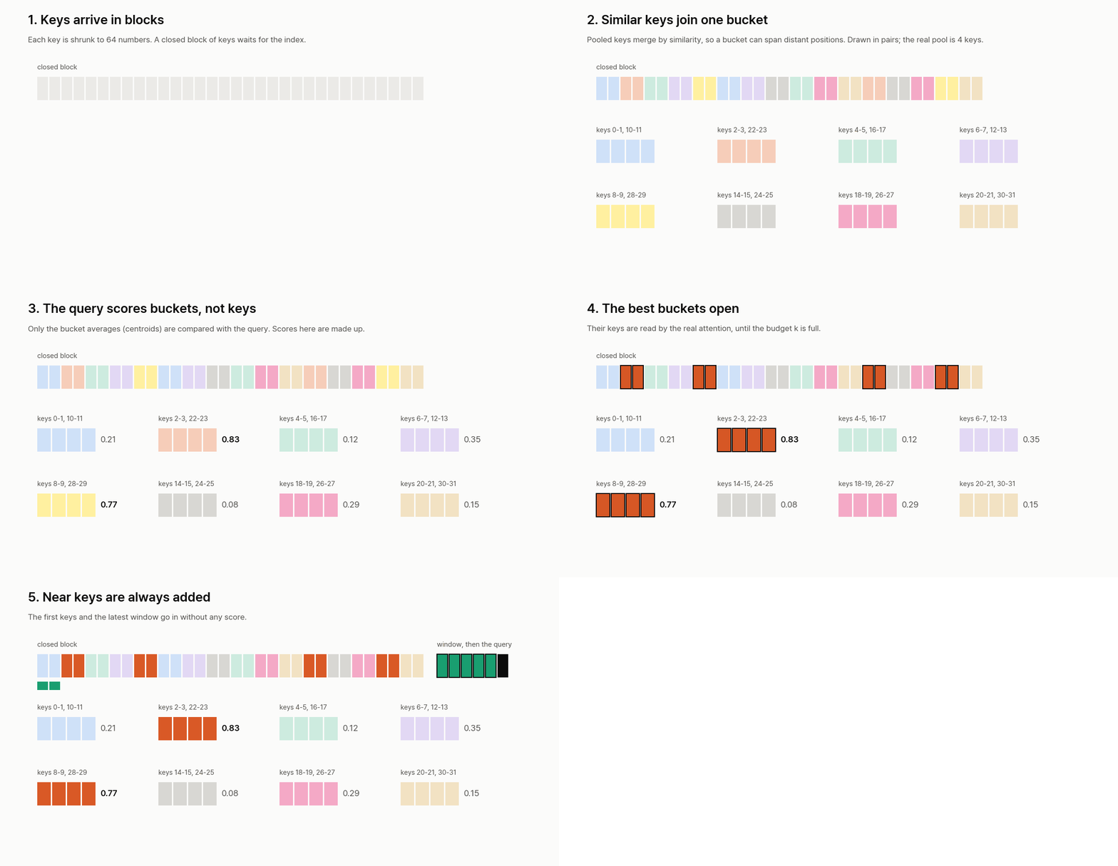
LSA puts buckets of similar keys in a small index space fitted to the model, so a query scores buckets and not keys. Its first keys and latest window are always read without a score. Our function is one query's flat search; it omits the pooling, the clustering and the tree search. The paper's headline figures are for 10M tokens on H200; our LSA post covers those, how they shrink at shorter contexts, and what we measured on a small index of our own.

• What improved. The paper reports 72.4x faster prefill than full attention in one Qwen3.8-27B layer at 10M tokens on one H200. The whole model on eight H200s gets 9.21x to the first token.
• Why it works. A query scores buckets and not keys. At 10M, by our calculation, that is about one eighth of a token scan's scores, while it still reads its 4,096 chosen keys.
• What it costs. It saves time and not memory, since the KV cache still grows with the context. Gains shrink at shorter contexts: the whole model's first token is 1.03x at 512K. On GLM-5.3-Flash, it trails that model's own sparse attention by up to 8 points at 2M to 5M, in a comparison the paper says favours the baseline, which was trained with the model.

def read_list(q, centroids, members, pos, top_p, k, window=512, sinks=4):
    """Which keys one query reads. q and centroids are unit vectors in the small index space."""
    near = set(range(sinks)) | set(range(max(0, pos - window), pos + 1))
    scores = centroids @ q                       # one score per bucket, not per key
    picked = scores.topk(min(top_p, len(scores))).indices
    far = []
    for b in picked.tolist():                    # open the best buckets first
        far += [key for key in members[b] if key not in near]
        if len(far) >= k:
            break
    return sorted(near | set(far[:k]))

Linear in length: no growing list to read#

The last group removes the source of the growing cost. Most of these never compare a query with a list of keys.

23. Linear Transformer (Katharopoulos, 2020)#

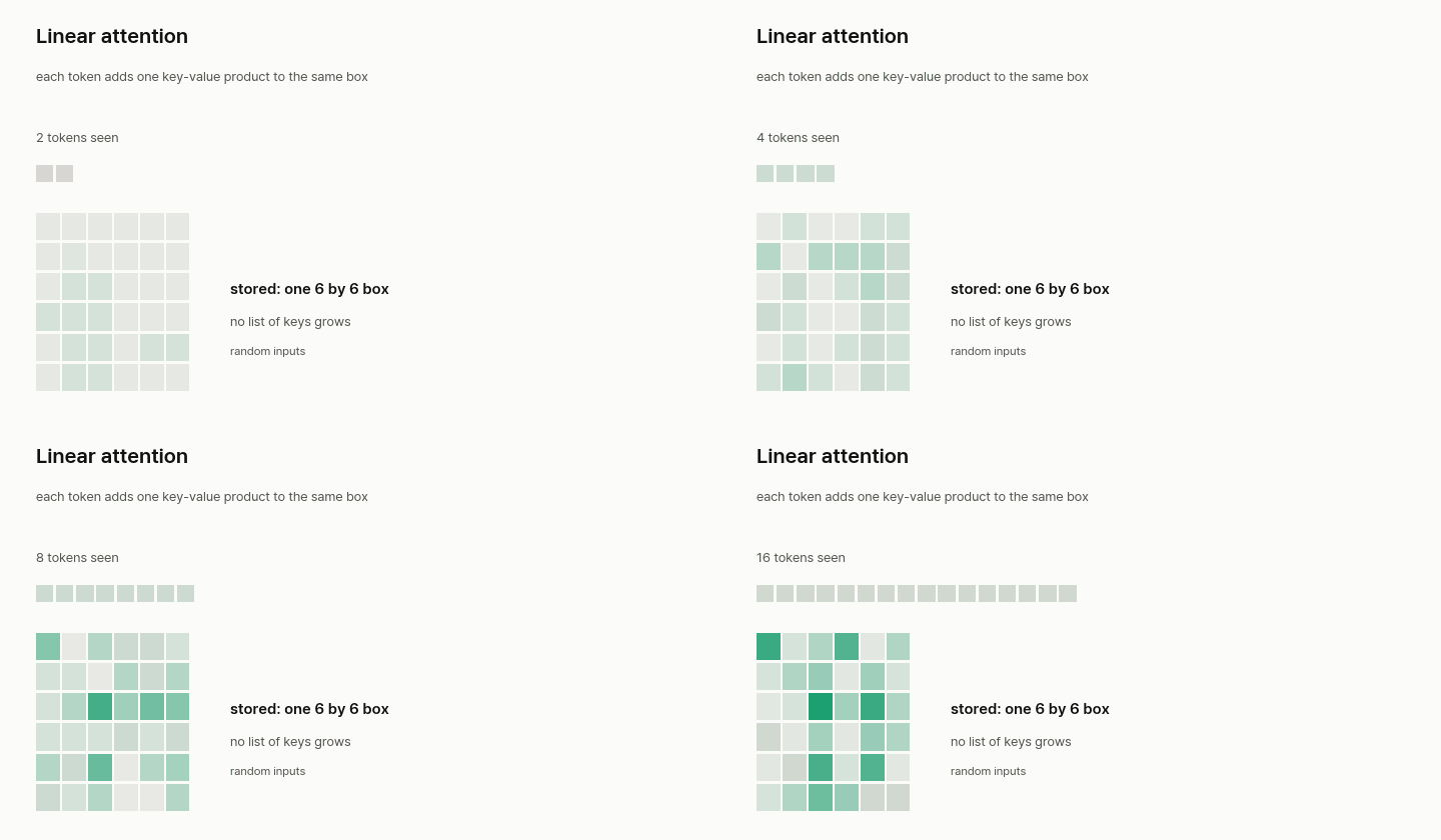
Transformers are RNNs swaps the softmax for positive features, which lets a running sum replace the list, so memory is constant at any length (the paper's recurrence). Our check confirms the recurrence returns the same output as the explicit causal sum. The GIF runs the same update on random inputs.

• What improved. Generation speed, by a huge margin. On CIFAR-10 it produces 17.85 images/s against 0.004 for softmax without a KV cache (4,462x) and 0.32 with one (about 56x, our calculation). After a one-week training budget it scored 3.40 against 3.47 bits/dim (lower is better).
• Why it works. A running sum replaces the list of keys, so each new token costs the same however long the sequence is.
• What it costs. Quality can drop. On WSJ speech, the validation phoneme error is 8.08 against 5.12 for softmax, at 824 against 2,711 seconds per epoch, so it is 3.3x faster and clearly less accurate. The Gated DeltaNet paper also says plain linear attention underperforms in language modeling.

def linear_attention(q, k, v):
    """elu + 1 keeps features positive, so a sum replaces the softmax. Memory stays fixed however long the input."""
    phi = lambda x: F.elu(x) + 1
    S, z, out = torch.zeros(k.shape[-1], v.shape[-1]), torch.zeros(k.shape[-1]), []
    for qi, ki, vi in zip(phi(q), phi(k), v):
        S = S + torch.outer(ki, vi)              # the state replaces the list of past keys
        z = z + ki
        out.append(qi @ S / (qi @ z))
    return torch.stack(out)

24. Linformer (Wang, 2020)#

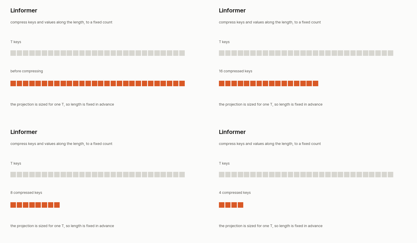
Linformer projects keys and values along the length down to a fixed c (the paper's k), independent of n, at O(nk). The projection is sized for one length, so the length is fixed in advance, which does not fit a cache that grows token by token.

• What improved. Time and memory, more as sequences get longer. At n=512 and k=128 it runs 1.5x faster for inference and fits 1.7x the batch. At n=65536 and k=128, it is 20x faster and uses 60x less memory (V100). At n=512, average classification accuracy is 91.75 at k=128 and 92.08 at k=256, against 92.25 for RoBERTa-base.
• Why it works. The paper finds that self-attention is close to low rank, so keys and values survive heavy compression along the length.
• What it costs. Quality depends on picking k, and the projection is sized for one n. Performer later adds that it is not causal and that it plateaus on PG-19.

def linformer(q, k, v, E, F_):
    """Compress T keys and values along the length to a fixed c. E and F_ are [c, T], so T is fixed in advance."""
    return attend(q, E @ k, F_ @ v)

25. Performer (Choromanski, 2020)#

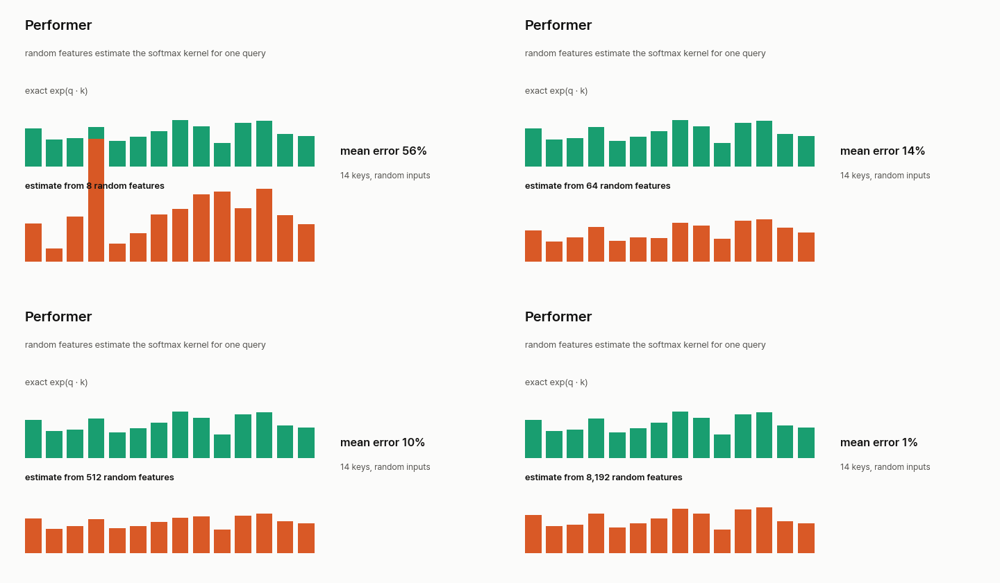
Performer estimates the softmax kernel with positive random features, so it can multiply the right pair first: O(Lrd) where full attention costs O(L²d). The paper rejects sine and cosine features, which go negative, so performer_features is its positive form (Lemma 1). The GIF is this function on our random small inputs, so its error is only an illustration. We omit orthogonal features, input rescaling and the causal version, which uses prefix sums.

• What improved. It keeps the softmax form and estimates it, where earlier fast designs added sparsity or low-rank assumptions. On TrEMBL at 36 layers, it matches the accuracy of exact softmax.
• Why it works. Positive random features turn the kernel into two factors, so the multiplication can run in the cheaper order.
• What it costs. Small errors travel across layers, so a very tight estimate may be needed. Weights moved over from a softmax model start at 0.07 accuracy and need a small amount of fine-tuning. On PG-19, positive features with redrawing are needed to match a Transformer, and sine and cosine features are unstable.

def performer_features(x, omega):
    """Positive random features whose dot product estimates the softmax kernel exp(x @ y). omega is [D, d]."""
    return (x @ omega.T - x.pow(2).sum(-1, keepdim=True) / 2).exp() / math.sqrt(len(omega))

def performer(q, k, v, omega):
    fq, fk = performer_features(q, omega), performer_features(k, omega)
    weights = fq @ (fk.T @ v)                    # multiply the right pair first: cost grows with T, not T squared
    return weights / (fq @ fk.sum(0, keepdim=True).T)

26. Mamba (Gu, 2023)#

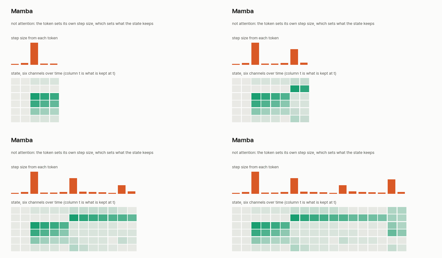
Mamba is no attention at all, and it is here because hybrids mix it with attention (our overview lists AI21's Jamba). Gu and Dao call it the "first linear-time sequence model" with Transformer-quality performance. A state-space model steps a fixed-size state forward, and the current token sets the step size and the input and output maps, so it decides what is kept. We show one channel with a diagonal A.

• What improved. Content-based reasoning, which the paper names as the weak spot of earlier state-space models. Mamba-2.8B scores a perplexity of 6.22 on The Pile (lower is better) and a benchmark average of 63.3, against 6.73 and 59.1 for Pythia-2.8B. Inference throughput is 4 to 5x a similar-size Transformer.
• Why it works. The current token sets the parameters, so the model chooses what to keep. With no KV cache to store, batches can be larger, and the paper credits that for the throughput.
• What it costs. Everything must fit in a fixed state, and the paper says that limits it. The Gated DeltaNet paper reports a retrieval average of 21.0 for Mamba against 37.0 for Transformer++, with inputs cut to 2K tokens.

We followed one sentence through a small Mamba hybrid, Granite-4.0-H-350M, in a separate post. With its four attention layers switched off, it still named the right person at 18 tokens, but at 1,410 tokens the probability fell to 0.002.

def mamba_step(h, x, A, B, C, delta):
    """A selective state-space step with diagonal A, one channel. The token sets the step size and also the
    input and output maps, so it decides what the state keeps and what gets read out. No attention at all."""
    d = delta(x)                                 # step size, from the current token
    a_bar = (d * A).exp()                        # zero-order hold of a diagonal system
    b_bar = (a_bar - 1) / A
    h = a_bar * h + b_bar * B(x)
    return h, (C(x) * h).sum(-1)

27. Gated DeltaNet (Yang, 2024)#

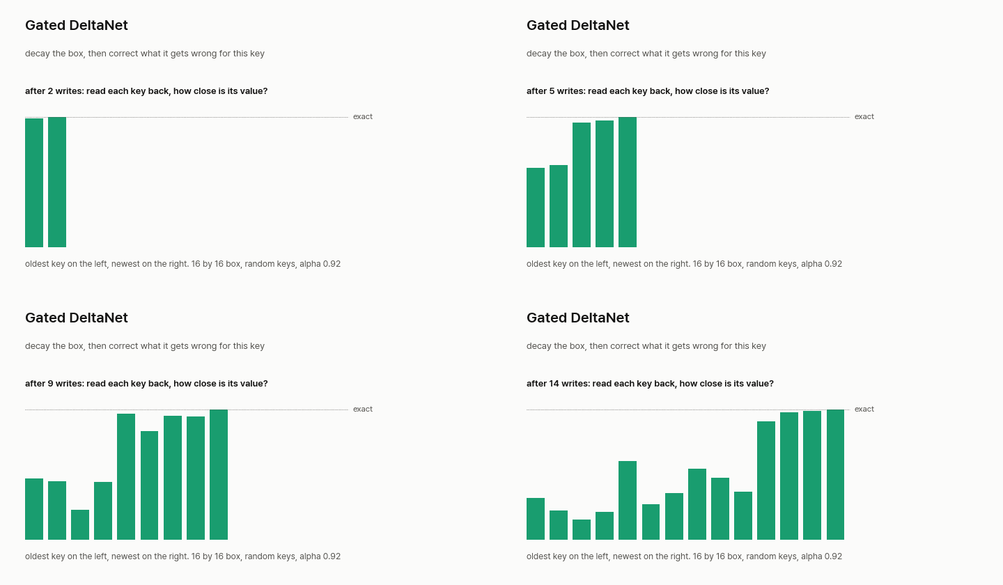
Gated DeltaNet keeps a fixed-size matrix. Each step decays it by alpha, then corrects what it gets wrong for this key, which makes the newest key read back well. The paper notes that alpha near 0 clears memory and alpha near 1 gives the pure delta rule, the update that only corrects the current error. The current Qwen hybrids in our overview use it next to some full-attention layers.

• What improved. Recall from a fixed-size state. In needle-in-a-haystack tests at 1.3B parameters, S-NIAH-2 at 4K scores 92.2 against 56.2 for Mamba 2 and 18.6 for DeltaNet, and S-NIAH-1 at 8K scores 91.8 against 30.4 for Mamba 2. DeltaNet does beat it there, at 98.8.
• Why it works. The delta rule corrects what the state gets wrong for this key, and the gate lets old content fade so new content has room.
• What it costs. A fixed state still runs out. S-NIAH-2 at 8K falls to 29.6, and the retrieval average is 30.6 against 37.0 for Transformer++. In the Kimi paper's table, GDN-H averages 51.2 against 52.2 for MLA, with all models given equal training tokens.

def gdn_step(S, k, q, v, alpha, beta):
    """Delta rule: S is a matrix of fixed size. Decay it by alpha, then correct what it gets wrong for this key."""
    S_kept = alpha * S
    S = S_kept - beta * torch.outer(S_kept @ k - v, k)
    return S, S @ q

28. Kimi Delta Attention (Kimi Team, 2025)#

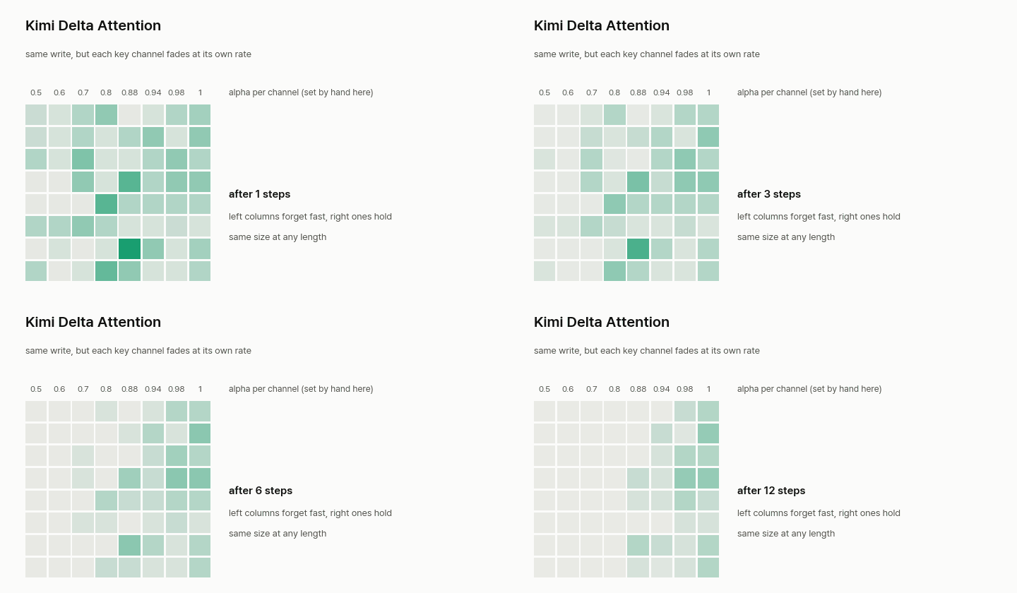
Kimi Linear keeps the same write, with a separate decay for each key channel, and reads with the plain query (Eq. 1). Keys and queries are L2-normalised, and the real layer adds an output gate (Eq. 10). The model mixes KDA and full MLA layers 3 to 1, and the paper reports that this reduces KV-cache use by up to 75%. Our check confirms that equal alphas return the same matrix as Gated DeltaNet.

• What improved. RULER at 128K is 84.3 against 81.3 for MLA and 80.5 for GDN-H, and the average is 54.5 against 52.2 and 51.2, all on 1.4T training tokens. At 1M tokens, the paper reports a 2.3x decoding speedup. Its headline figure, 1.84 against 11.48 ms per output token for MLA (6.3x), it calls theoretical and credits to the larger batches this design allows, so that figure is not a single-request speed.
• Why it works. Key channels get their own decay, so some can hold on to far context while others forget quickly.
• What it costs. The full MLA layers have to stay, because the paper finds long-context retrieval is the bottleneck. Not every long-context test improved either: LongBench V2 is 35.0 against 36.1 and Frames is 58.8 against 60.5.

def kda_step(S, k, q, v, alpha, beta):
    """Kimi Delta Attention: Gated DeltaNet's write, but alpha decays each key channel at its own rate.
    q and k are L2-normalised."""
    S_kept = S * alpha[None]                     # decay keeps channels independently
    S = S_kept - beta * torch.outer(S_kept @ k - v, k)
    return S, S @ q

What to ask when a new model card appears#

These four questions place every design in this post, and they are a good start on a new one:

1. What is stored per token? One full key and value per head, per group, one small vector, or nothing but a fixed box.
2. Which keys can a query read? All of them, a fixed mask, or a chosen subset.
3. If chosen, what gets scored? Every key, every block, or a group made by content.
4. Which layers does this apply to? Many of the models above mix designs across layers, so one label rarely describes a whole model.

What we checked and what we did not#

Run on CPU. Output shapes; no reading the future for the causal masks; Luong's general form with an identity matrix matching the dot form; GQA matching MHA and MQA at its two ends; a large sliding window matching the full causal mask; the sink mask's key count and first keys; local-global layers switching between the window and the full mask; Sparse Transformer's two-hop reach; Longformer's symmetry, window and global rows; BigBird only adding keys to Longformer; block scan reading only winning runs; Reformer reading itself only when alone; the key counts under ClusterKV's and LSA's budgets; linear attention's recurrence against its explicit sum; Performer's estimate against the true kernel on small inputs; the delta-rule write being exact with alpha=1, beta=1; and Kimi Delta Attention with equal alphas matching Gated DeltaNet.

Read against the source. Each function was compared with its paper, and each entry above states what it leaves out. Sliding window and local-global layers have no single source. Block scan rests on the LSA paper's description alone.

Not done. No design here was trained, no speed or accuracy figure was reproduced, and the functions leave out the optimized low-level routines that make the real ones fast. Nothing in this post tells you which design is best for your model. For what each design costs on current models, with their real config values, read the overview of seven designs.