Latent Sparse Attention: 72x in One Layer, 9x for the Whole Model at 10M Tokens
The paper reports 72.4x prefill in one Qwen3.8-27B layer and 9.21x to first token for the whole model at 10M tokens, with almost no first-token gain at 512K. We follow real queries through a small LSA index on Qwen3-8B to show how it did, what its limits are and what it missed. We did not run the LSA server.
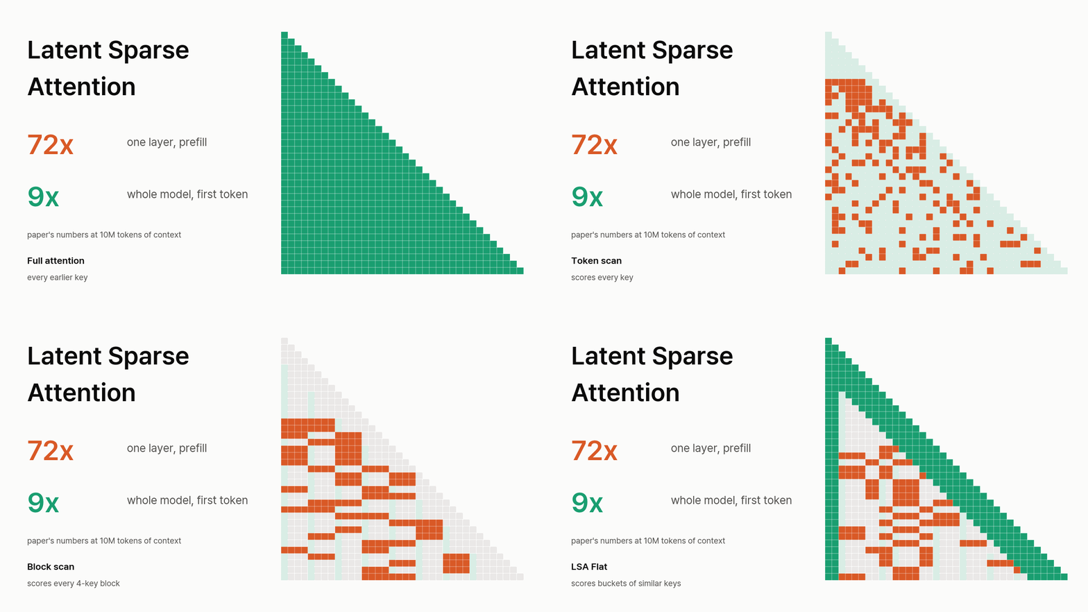
Latent Sparse Attention: 72x in One Layer, 9x for the Whole Model at 10M Tokens
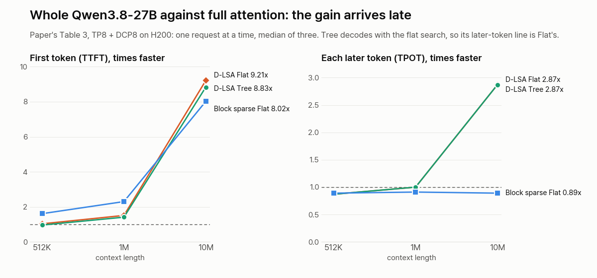
Latent Sparse Attention (LSA) is a new attention design from Kubicek et al. at Prefrontal AI and ETH Zurich. The paper reports that at a 10-million-token context, one attention layer of Qwen3.8-27B runs 72.4 times faster than full attention in prefill (reading the context in) and 42.5 times faster in decode (producing each new token). For the whole model on eight H200s, the first token drops from 4,582 seconds, about 76 minutes, to about 8 minutes, which is 9.21 times faster.
That gain arrives late. At 512K tokens the same table shows 1.03x for the first token, at 1M it shows 1.51x, and each later token is no faster at 1M. The table has nothing between 1M and 10M, so do not expect these numbers away from about 10M.
The idea fits in one example. Sparse attention reads only some earlier tokens, so something has to choose them. LSA sorts earlier tokens into buckets by similarity, and a new token scores the buckets, not the tokens. When we built a simplified version of that index on Qwen3-8B, one bucket held Author: Jane Aust from the Gutenberg header and Jane Aust from the title page 196 tokens later. Another held query_count: int and query_count: Number from a Python file.
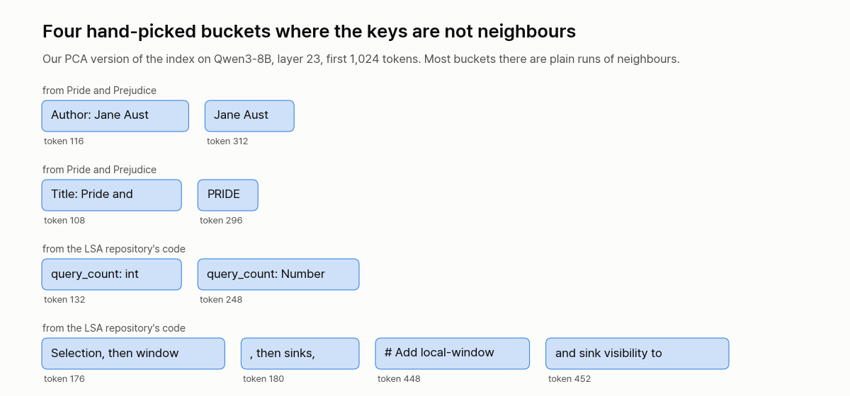
We picked these because they stand out. In the first 1,024 tokens at layer 23, most buckets were plain runs of neighbouring tokens: 95, 74 and 93 of 128 in our three documents.
This post starts with the cost LSA goes after and follows one real query through the index. Then it covers what is good about the design, what its limits are and what our own test showed. We did not run the LSA server, so we have no speed number of our own. (Unrelated: LongCat Sparse Attention is also abbreviated LSA. This post means the Prefrontal design.)
Why choosing costs so much
In attention, each new token asks a question, called the query, and every earlier token carries a label, called the key. Full attention compares the query with every key, so at 10M tokens one new token makes 10M comparisons.
Sparse attention reads a fixed number of keys instead, say 4,096. That makes the read cheap, but someone still has to choose those 4,096. The part that does this is called the indexer.
There are three broad ways to choose, and they differ in how many scores one query makes. At 10M tokens:
- A token scan scores every key: 10M scores.
- A block scan scores each run of 4 adjacent keys: 2.5M.
- LSA scores each bucket of about 8 keys: about 1.25M.
These three figures are 10M divided by the group size. LSA has two search modes. Scoring every bucket, as above, is called Flat. Arranging the buckets in a tree and scoring only some paths through it is called Tree. Whole-model numbers and our own test in this post are Flat unless we say otherwise.
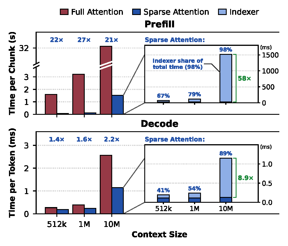
The paper shows why the number of scores matters. In one GLM-5.3-Flash layer at 10M tokens, the indexer takes 98% of sparse attention's prefill time, and the authors calculate that a free indexer would make prefill another 58 times faster and decode 8.9 times faster (one H200). So LSA goes after the choosing, not the reading.
Below is the paper's Figure 2 (Kubicek et al., CC BY 4.0). In the small charts on the right, the light blue part is the indexer, and it takes most of sparse attention's time as the context grows.
One real query, start to finish
Fewer scores could also mean missing more. To see what happens, we follow one query through the small index we built: Qwen3-8B, Pride and Prejudice, layer 23.
The query we follow is token 23,711 of the novel. A model reads words in pieces called tokens, and the name Bingley becomes three: B, ingle and y. Our query is the y at the end of "...if Miss Bennet were not decidedly better. Bingley", the moment the model has just finished writing the name.
We picked it for being ordinary. We tested 1,024 queries in this document and took the one where LSA's lead over its comparison (the block of 8, introduced below) is exactly in the middle. The point is not to show only a case that went well.
What the query wants. Some keys never need choosing: the first 4 in the document and the latest 512 are always read without a score. So the keys that actually have to be chosen are the 23,195 in between. In this post, the attention a query gives to those 23,195 is called far attention.
This query's far attention is concentrated. Count all of it as 100, and 62.6 goes to just 8 keys. Six are ingle, the middle piece of earlier mentions of Bingley. Two are Aust from "Miss Austen" in the book's preface. Having just written Bingley, the model looks back at the earlier Bingleys. So a good method has to find these 8 among the 23,195.
Three ways to find them, each allowed 256 keys. We grade each by how much far attention the keys it read hold, and call that coverage: 0.40 means 40%. We cut the block scan to runs of 8 here, which we call a block of 8. That brings its number of scores close to LSA's, so we can see who finds more for the same effort.
- A token scan scores all 23,195 keys. It finds all 8, with coverage of 0.771.
- A block of 8 makes 2,899 scores. It finds 2 of the 8, with coverage of 0.217.
- LSA scores 2,944 buckets, then opens 35 of them, best first, until it has 256 keys. The first three are
Bingley followed,ingley had not, and a bucket holding bothBingley wasandingley92 tokens later. It finds 5 of the 8, with coverage of 0.401.
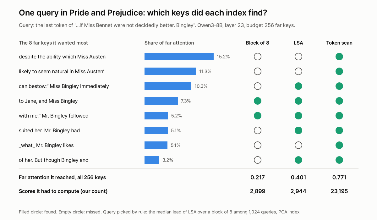
So with about the same number of scores, LSA got nearly twice as much as the block of 8, and with about one eighth of the scores it got about half of what a token scan got. Our reading of why: the bucket's average mostly describes Bingley, while a block of 8 averages the name with whatever words surround it. We did not test that explanation.
LSA also missed things. Both Aust keys, the two largest shares, and one ingle stayed closed. Those three hold 31.5% of far attention, and only the token scan reached them. A bucket's score stands in for its members, so a key is never looked at unless its bucket scores well enough. That is the price of making fewer scores.
The same steps in general
What just happened to that query comes down to five steps. The first two happen ahead of time as keys arrive, and the last three happen for each query.
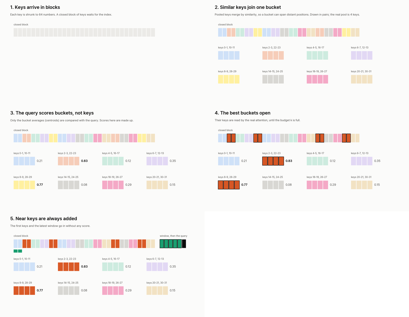
- Shrink. Each key is projected down to 64 numbers. These small keys exist only for choosing.
- Group. Each block of 512 keys is pooled in fours and merged by similarity (Ward clustering) into buckets of about 8 keys, 16 at most.
- Score. The query, also shrunk, is compared with each bucket's average, called a centroid.
- Open. The best buckets contribute their keys until the budget is full. On Qwen3.8-27B that is 4,096 keys.
- Add the nearby keys. The first 4 keys and the latest 512 are always read. The real attention then runs over this list.
Here are steps 3 to 5 as a short function. We wrote it to test our understanding and ran it once on made-up vectors. The repository's real version is decode_flat, which works on batches.
def read_list(q, centroids, members, pos, top_p, k, window=512, sinks=4):
    """Which keys one query reads. q and centroids are unit vectors in the small index space."""
    near = set(range(sinks)) | set(range(max(0, pos - window), pos + 1))
    scores = centroids @ q                       # one score per bucket, not per key
    picked = scores.topk(min(top_p, len(scores))).indices
    far = []
    for b in picked.tolist():                    # open the best buckets first
        far += [key for key in members[b] if key not in near]
        if len(far) >= k:
            break
    return sorted(near | set(far[:k]))
The window is set to one block of 512 keys so that it covers every key not yet clustered. A key from an opened bucket that already falls in the window or the first 4 is skipped, and the next one takes its place.
There are three ways to make the small keys in step 1. The headline speed numbers come from the first, and our test mainly uses the second.
- D-LSA freezes an already-trained model and trains only the two small projections and a temperature per layer, so that the index imitates the model's real attention. The paper uses 352M tokens and 48,000 steps. The weights are release assets of the repository.
- D-LSA (Training-Free) uses PCA in place of training.
- N-LSA trains a new model with LSA built in. The paper tests this on a model of about 0.5B parameters, not on Qwen.
Contribution
From here on, these are the paper's results. Lined up against the existing designs, LSA's place is easy to see.
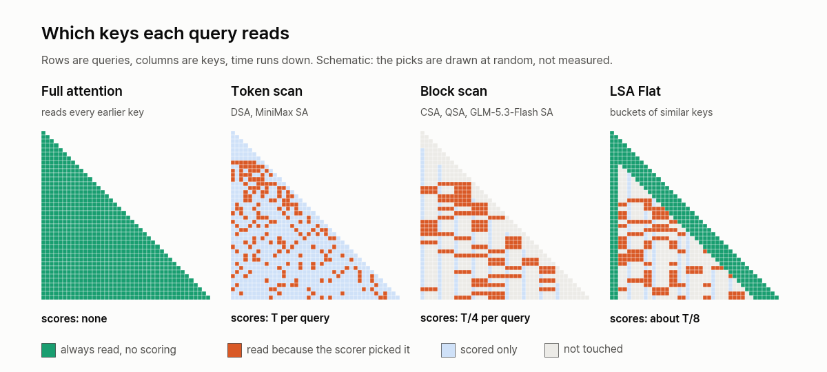
| Design | What a query scores | Scores per query | What it reads |
|---|---|---|---|
| Full attention | Nothing | None | Every earlier key |
| Sliding window | Nothing | None | The latest keys, older ones are gone |
| Token scan (DSA, MiniMax SA) | Every key | T | The best keys |
| Block scan (CSA, QSA, GLM-5.3-Flash SA) | Every run of 4 adjacent keys | T/4 | The best runs |
| Earlier semantic methods (ClusterKV, RetroInfer) | Every centroid of clustered keys | Fewer than T, still grows with T | Keys of the best clusters |
| LSA Flat | Every bucket | About T/8 | Keys of the best buckets |
| LSA Tree | Nodes on a beam-search path | Grows with log T | Keys of the best buckets |
T is the number of earlier keys.
It cuts the cost of choosing and keeps the read. At 10M tokens, one query makes about one eighth of a token scan's scores and about half of a block scan's, while still reading its 4,096 chosen keys. That takes some extra storage for the buckets, but not much: on GLM-5.3-Flash at 10M tokens, the paper reports a 246 MiB bucket cache beside 10 GiB of KV cache per layer.
At 10M tokens, producing new tokens gets faster too. In the whole model, tokens after the first are 2.87x faster than full attention. In the same comparison a block scan is 0.89x, slightly slower. The two also read different numbers of keys (2,048 for the block scan, 4,096 plus the first and latest keys for LSA), so this is not the design's effect alone.
A bucket can hold keys that are not neighbours. A block scan's groups are whatever happens to sit together, while LSA groups keys by similarity. In our query above, LSA found 5 of 8 wanted keys against 2 for the block of 8. We did not test whether separated keys are the cause, though, and its first two opened buckets are plain runs.
The grouping is fitted to what the model looks at. Grouping by content is not new. ClusterKV and RetroInfer do it, and the paper describes them as training-free, inference-only methods, none evaluated above 1M. D-LSA trains the small keys against the model's own attention.
On Qwen, the speed does not obviously cost accuracy. Faster is no use if the answers get worse, so this result matters. Qwen3.8-27B with LSA Flat stays within 5 points of full attention up to 1M tokens on RULER, a long-context test, and on the paper's own PaperTrail set. At 10M it scores above full attention on both, RULER 63.9 against 59.9 and PaperTrail 29.1 against 19.8, but the sample there is thin, which we come back to under the limits.
Why 72x in one layer becomes 9x in the model
At the same 10M tokens, 72x in one layer shrinks to 9x in the whole model. There are two likely reasons.
The first is the paper's stated reason. LSA speeds up only the global attention layers, and the other layers keep their cost.
The second is our guess. The 72x is measured only on the last chunk before the 10M mark (32,768 queries), while a real prefill also passes through all the shorter contexts, where the gain is smaller. The paper's GLM-5.3-Flash numbers show the same trend: the gain in one layer over GLM's own sparse attention rises from 2.1x at 512K to 22.7x at 10M. We did not measure how much each reason contributes.
The chart below is the whole model, serving one request at a time. Its "block sparse Flat" is what this post calls a block scan.
That 9x is also against full attention. GLM-5.3-Flash already uses sparse attention, so its gain is much smaller. With the KV cache split across eight GPUs by token, the first token at 10M is 2.24x faster and later tokens 2.10x, and up to 1M neither passes 1.09x.
Limits
Below about 1M tokens the gain is small. Against full attention, the first token is only 1.03x faster at 512K and 1.51x at 1M. In the same range a block scan gives 1.61x and 2.30x, faster than LSA. LSA takes over only at 10M, 9.21x against 8.02x. As noted above, LSA reads more keys in this setup, so this is not the design's effect alone. Later tokens at 512K are slightly slower than full attention for both LSA and the block scan (0.87x to 0.89x).
It saves time, not memory. LSA reduces the cost of finding keys, not of storing them. The paper says so directly: the KV cache still grows linearly with the context. So at 10M tokens GLM still needs 10 GiB of KV per layer.
Flat keeps getting more expensive as the context grows. Its scores drop to T/8, but that still grows with T. Tree is the answer to this, with scores growing only with log T, but it has costs for now. For the whole model's first token at 10M it is 8.83x against Flat's 9.21x, and the paper predicts Tree passes Flat in prefill only beyond 10M. On GLM's RULER at 10M, Flat scores 66.8 and Tree 55.8.
A bucket only gathers keys within one 512-key block. The clustering runs block by block. The keys our query wanted were spread from token 1,827 to 21,460, so even identical ingle keys cannot share one bucket, and the query has to open each separately. The design does not find one name scattered across a whole book in one go.
The strongest accuracy result has the thinnest sample. That is the high 10M score above. Each task uses 100 prompts up to 1M and 20 past it, and about 2.7 of RULER's 4.0-point gap comes from 2 of its 13 tasks (MultiQuery 92 against 72, HotpotQA 35 against 20). Qwen also only reaches 10M with its position encoding stretched by YaRN, a factor of 40 (42 for PaperTrail). On GLM, LSA Flat stays within 3 points of its sparse baseline up to 1M and trails by up to 8 at 2M to 5M, though the paper adds that this comparison favours the baseline, which was trained together with the model.
Training a new model with it is still small. The paper trains N-LSA at about 0.5B parameters, up to 128K tokens and with flat search only, and leaves larger models and tree search open. Peak memory is also about 1 GiB higher per layer at 128K tokens, partly because the selected indices are kept for the backward pass.
What our test showed
The paper's tables give speed and answer accuracy. They do not say how much of the attention a query wanted it actually gets when it opens buckets, as we saw with the query above. So we measured coverage at a larger scale.
The setup is small and different from the paper. We ran Qwen3-8B on an A100 over three documents of 32,768 tokens each (the LSA paper, code from its repository, Pride and Prejudice), with 1,024 queries from the second half of each. We reimplemented the index from the paper's Algorithm 1 and did not use their code. We scored four budgets from 256 to 2,048 far keys, which gives 36 cells: 3 documents, 3 layers, 4 budgets. We compared LSA with the block of 8, a block of 4, which makes twice LSA's scores and is what real block scans use, a token scan, which makes eight times as many, and the best possible, which simply takes the keys with the most attention.
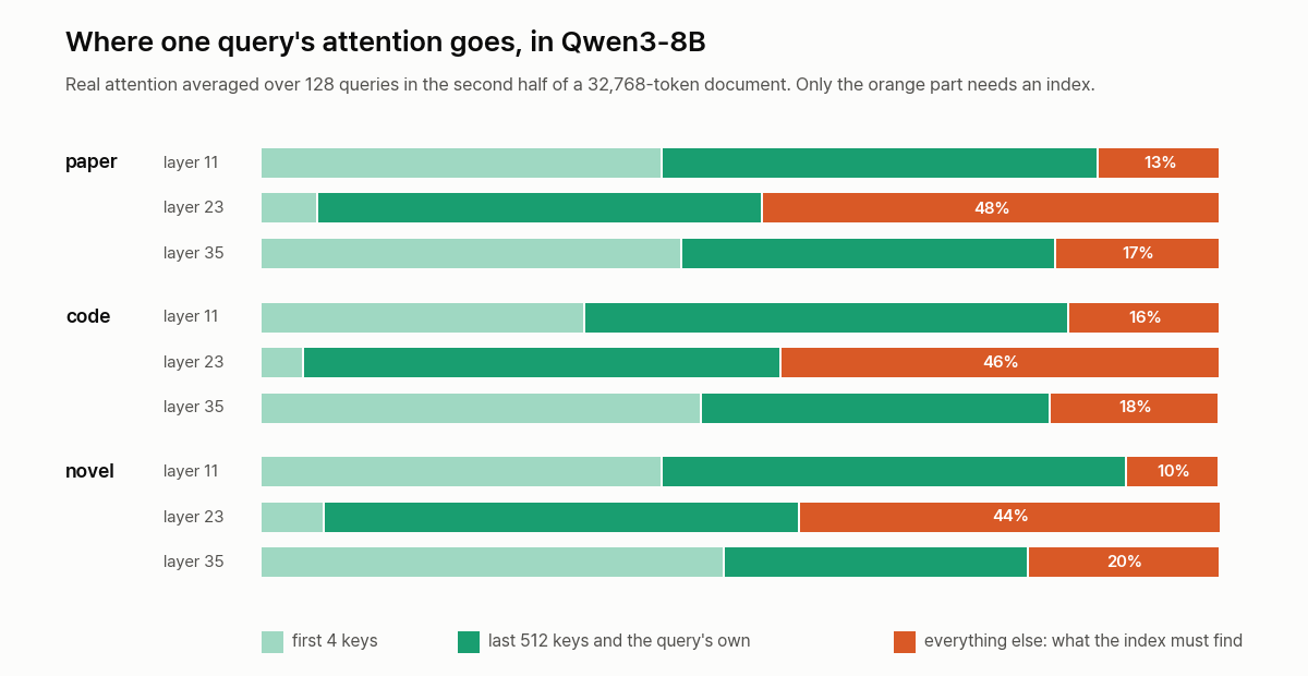
The amount there is to choose differs a lot by layer. Over 128 queries, at layers 11 and 35, only 10% to 20% of attention goes to far keys. The first 4 keys and the latest 512, read without a score, take the rest. Layer 23 is at 44% to 48%. So the results below split into layer 23 and the others.
For the same number of scores, LSA found more than a block of 8, but the gap was large only at layer 23. This is without training, with small keys made by PCA (fitted on the two other documents).
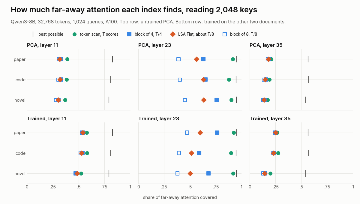
- LSA beat a block of 8 in all 36 cells (paired bootstrap, 95% interval above 0). The gap is 0.11 to 0.23 at layer 23 and at most 0.021 at layers 11 and 35.
- A block of 4 and a token scan, which make more scores, each beat LSA in all 36 cells. These two are point estimates without an interval, and the smallest gap is 0.0012.
- At layers 11 and 35 every method stays far from the best possible. On the novel's layer 11 at 2,048 keys: token scan 0.370, block of 4 0.305, LSA 0.302, block of 8 0.280, best possible 0.793.
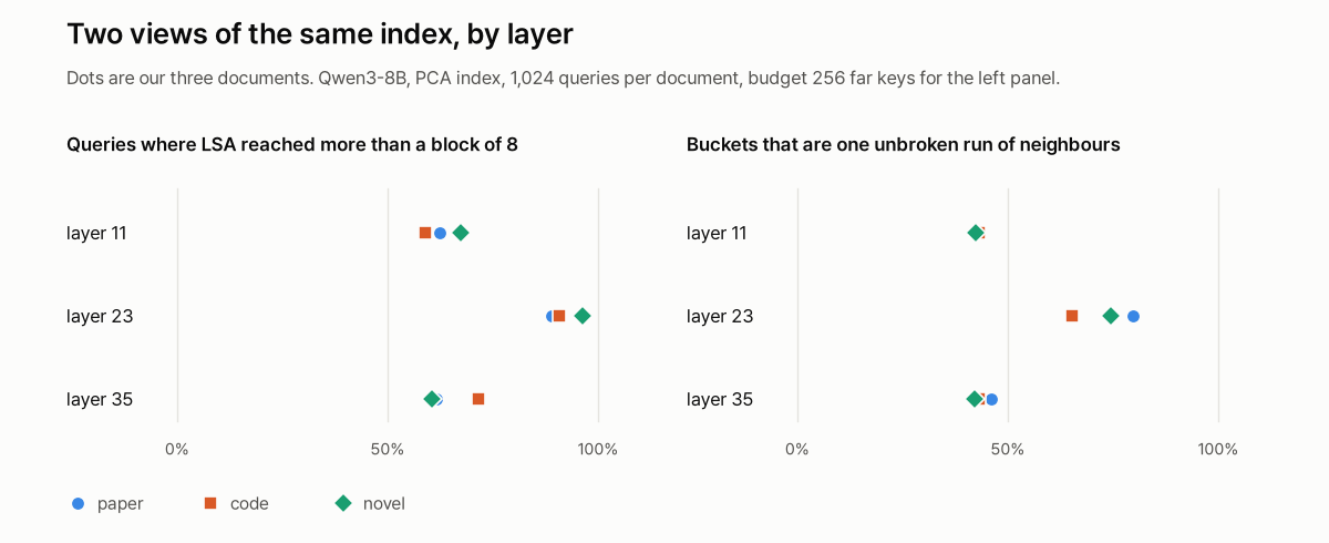
Query by query, the picture is the same. After those results we looked at each query at a budget of 256, the smallest. At layer 23, LSA reached more than a block of 8 on 89% to 96% of queries. At layers 11 and 35 it did on 59% to 72%, with a median lead of only 0.001 to 0.007, and the block of 8 won the rest.
Here is what so small a gap looks like. Take a middle query at the novel's layer 11: the and in "...delight in overthrowing those kind of schemes, and". The 8 keys it wants most hold only 4.6% of far attention between them, and no key is above 1%. Coverage is 0.024 for LSA, 0.017 for the block of 8 and 0.060 for the token scan. Unlike our first query, it has no concentrated keys, so no method has a clear target. That is one query, and we did not measure this pattern across all queries.
Similar to a person is not the same as wanted by the model. Back at layer 23 in the novel, take a query at the 10th percentile of LSA's lead: the comma after "They all paint tables, cover screens," in a conversation about accomplished young ladies. The first buckets LSA opened were otch and Irish airs, and singing too long in public and sentiments, of playing. To us those look on topic. But real attention wanted the same names again, Bingley and Austen, with 72.2% of far attention on 8 keys. LSA found 1 of them and reached 0.137. A token scan found all 8 and reached 0.843.
Buckets with separated keys were not common. We counted how many buckets look like the Jane Aust one at the top. Over our whole 32,768-token documents, buckets that are one unbroken run of neighbours make up 65% to 80% at layer 23 and about 43% at layers 11 and 35. Even when a bucket does split, the median distance from its first key to its last is 24 to 32 tokens at layer 23 and 60 to 132 at layers 11 and 35, so Jane Aust at 196 tokens is on the far side of typical.
Training the small keys gave mixed results. The gap between what looks similar and what the model wants is the problem the paper's training targets, so after those results we added a small training run. We followed the paper's Equation 2 on the two other documents, but at a far smaller scale: 65,536 tokens and 1,500 steps, against 352M tokens and 48,000 steps. The temperature starts at a fixed -3.0 rather than the paper's per-layer calibration. So this does not grade the paper's training. The trained projections were applied to the token and block scans too, so all of them are compared in the same space.
- Layers 11 and 35 improved on average: LSA's coverage rose 0.055 to 0.223 at layer 11 and 0.001 to 0.083 at layer 35. We did not compute paired intervals for these gains. The block of 8 rises too: on the novel's layer 11 at 2,048 keys it goes from 0.280 to 0.471, while its gap to LSA narrows from 0.021 to 0.016.
- LSA passed a block of 4 in 6 of those 24 cells, by point estimate, and it still never passed a token scan.
- Layer 23 got worse on two of three documents, by as much as 0.178 on the novel.
At layer 23, attention piles onto a few keys. This may relate to why this layer's results stand apart. Eight keys hold 54% to 69% of its far attention averaged over 128 queries, against under 1% at the other two layers. In the novel, all eight are Aust or ingle, the same keys our two example queries wanted. This is not document-start behaviour, since those keys sit at tokens 1,827 to 21,460. We did not test whether this is why buckets lag here or why training hurt.
What this does and does not say about the paper. It cannot confirm or contradict 72x. Our run is one small model, 32K tokens not 10M, a far smaller training set, attention coverage not answer accuracy, and no timing. Qwen3 also rotates all key dimensions with its position encoding, where the paper notes Qwen3.8 rotates a quarter, and our index reads keys before that rotation while its target is the rotated attention. We did not test that effect either. What it does show is what the grouping trades away at this scale: for the same number of scores it finds more than adjacent blocks do, and it finds less than scanning more.
If you want to try it
From the repository (Apache-2.0), which we read at commit 97b82d6 and did not run. Serving uses a fork of SGLang, the image ghcr.io/prefrontal-ai/sglang:lsa-v0.1.0, with --attention-backend fa3 --page-size 1 --disable-prefill-cuda-graph. LSA is not in that image, so the README has you install the repository into it. The server log must print armed; without that line, the server is running the checkpoint's own attention. The projection weights are .pt files in the release d-lsa-weights-v1, and the base model comes separately.
The fast kernels are written in CuTe DSL for H200 and B300, and Triton versions are not tied to those GPUs. The paper's Table 11 lists 17.41 ms in CuTe and 39.48 ms in Triton on H200, for one Flat prefill chunk of 32,768 queries at 10M, with synthetic inputs and kernel time alone. The README's reproduction run for one H200 is Qwen Flat on RULER at 4K and 32K, listed at 0.974 and 0.968 against the paper's 0.975 and 0.966, with a wall time of 1 h 52 min. That checks an install and is not a 10M run.
What we did not check
We did not serve the model, did not download the weights, and did not reproduce any speed or accuracy figure from the paper. Every H200 number above comes from the paper or its README, and we give no B300 numbers. The 4,582-second row is one request on one machine setup, so a busy server may behave differently.
For the seven older designs, including token and block scans, start with our attention overview, or the code version if you want them as short functions.
To see LSA next to 27 other attention designs, drawn the same way, read 28 Attention Designs, Each With a GIF and a Short Function.